


 客服




综合解决方案提供 10 MHz 至 3.6 GHz 的频率范围
多点触控界面
包括频谱分析仪和 IQ 分析仪(基础)模式
内置标配选件包括 P03、PFR、FSA、NFE 和 B25
N 型(阴头)输入连接器
与 SNS 系列噪声源兼容:N4000A、N4001A、N4002A
包括 U7227A 10 MHz 至 4 GHz 外部 USB 前置放大器
ONETEST 欢迎您
厂商登录 | 入驻
登录 | 注册 购物车 微信公众号厂商登录
类似产品
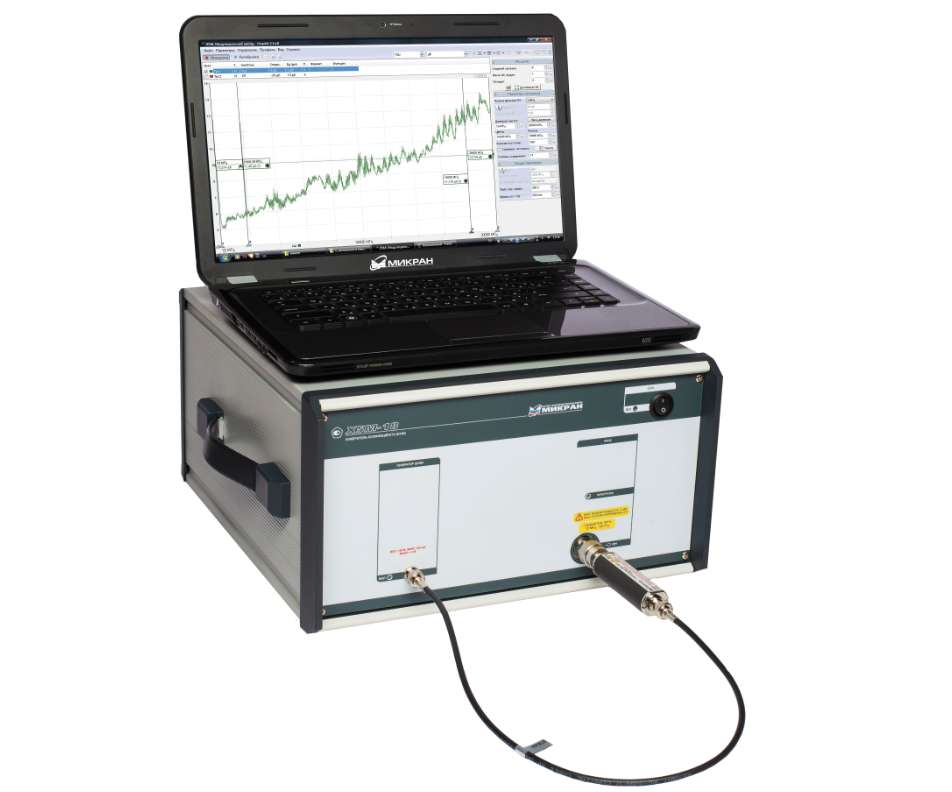
频率范围:10 MHz至4/20 GHz噪声比和增益测量使用固定或外部异源转换器进行测量内置恒温YIG预选器测量速度快使用特殊的下变频器单元将 NFA 解决方案扩展到 50 GHzSCPI 语言兼容性
SP926N(10MHz~26.5GHz)频率范围:10MHz~26.5GHz测量带宽:8MHz分析带宽:40MHz噪声系数仪器不确定度:±0.02dB测量/模式切换速度:75ms

10 MHz 至 50 GHz(可扩展至 110 GHz)· 噪声系数 0–30 dB · 测量不确定度 ±0.15 dB
同厂商产品
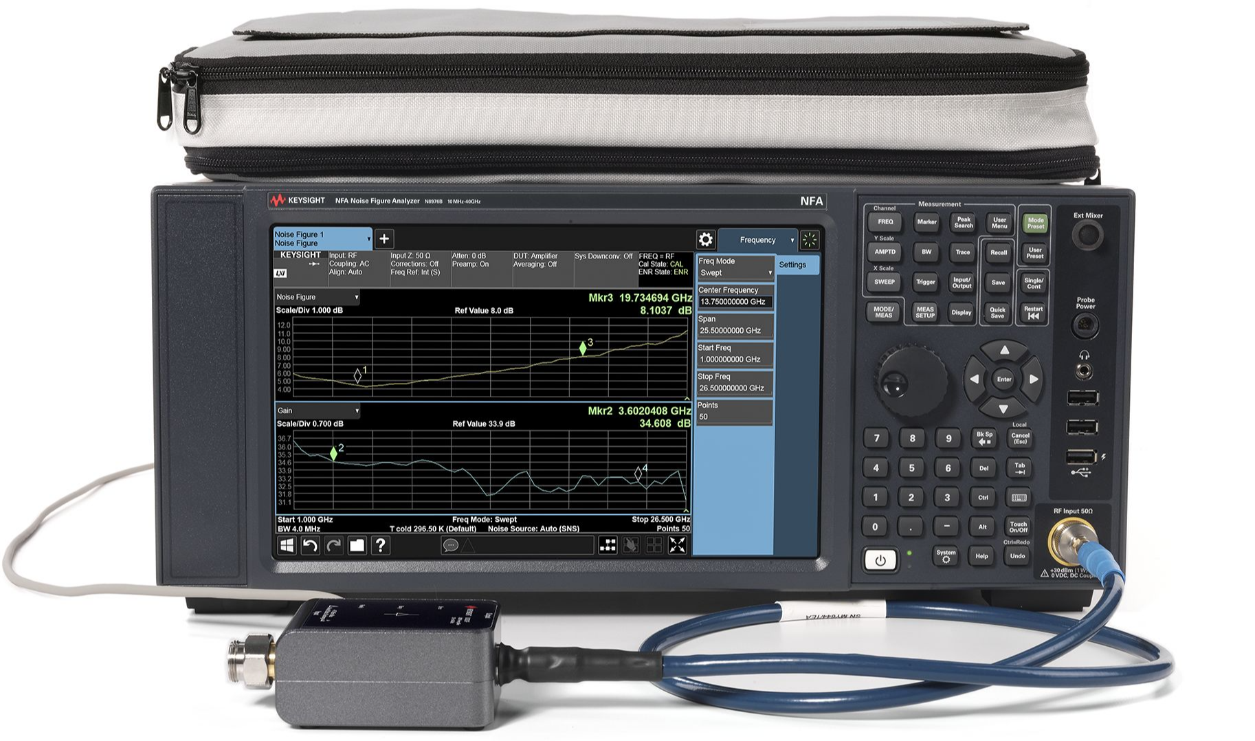
一体式解决方案,频率范围为 10 MHz 至 40 GHz多点触控界面包括频谱分析仪和 IQ 分析仪(基础型)模式内置标配选件包括 P44、PFR、FSA、NFE 和 B252.4 mm(阳头)输入连接器SNS 系列噪声源兼容性包括 U7227F 2 GHz 至 50 GHz 外部 USB 前置放大器和 346CK40 1 GHz 至 40 GHz 噪声源
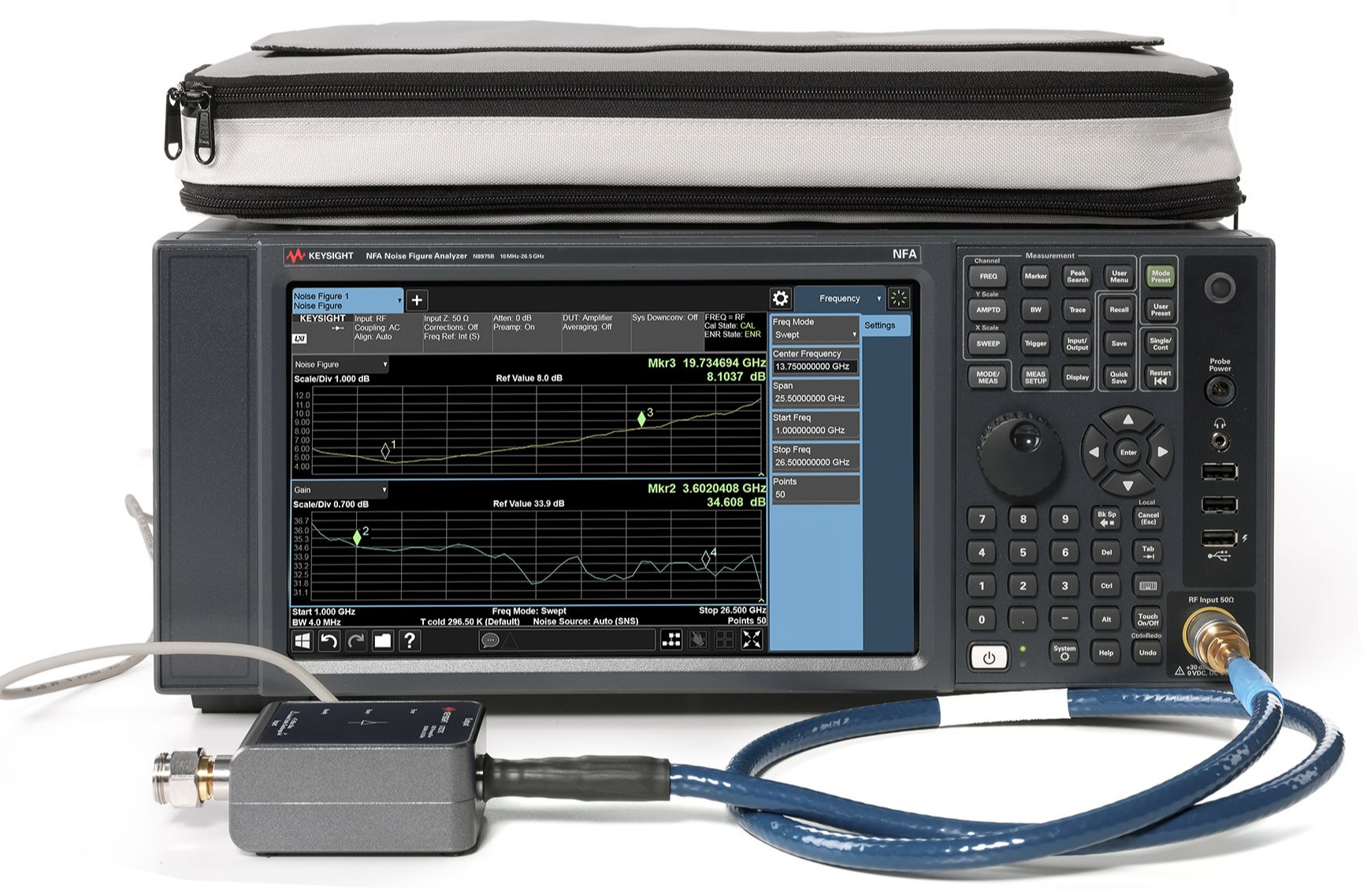
在一体化解决方案中提供 10 MHz 至 26.5 GHz 频率范围多点触控界面包括频谱分析仪和 IQ 分析仪(基础型)模式内置标配选件包括 P26、PFR、FSA、NFE 和 B25N 型(阴头)输入连接器SNS 系列噪声源兼容性包括 U7227C 100 MHz 至 26.5 GHz 外置 USB 前置放大器
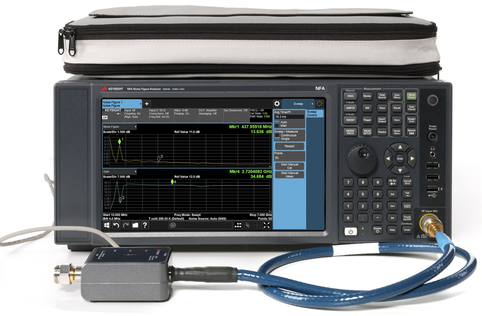
综合解决方案提供 10 MHz 至 7 GHz 的频率范围多点触控界面包括频谱分析仪和 IQ 分析仪(基础)模式内置标配选件包括 P03、PFR、FSA、NFE 和 B25N 型(阴头)输入连接器与 SNS 系列噪声源兼容:N4000A、N4001A、N4002A包括 U7227C 100 MHz 至 26.5 GHz 外部 USB 前置放大器
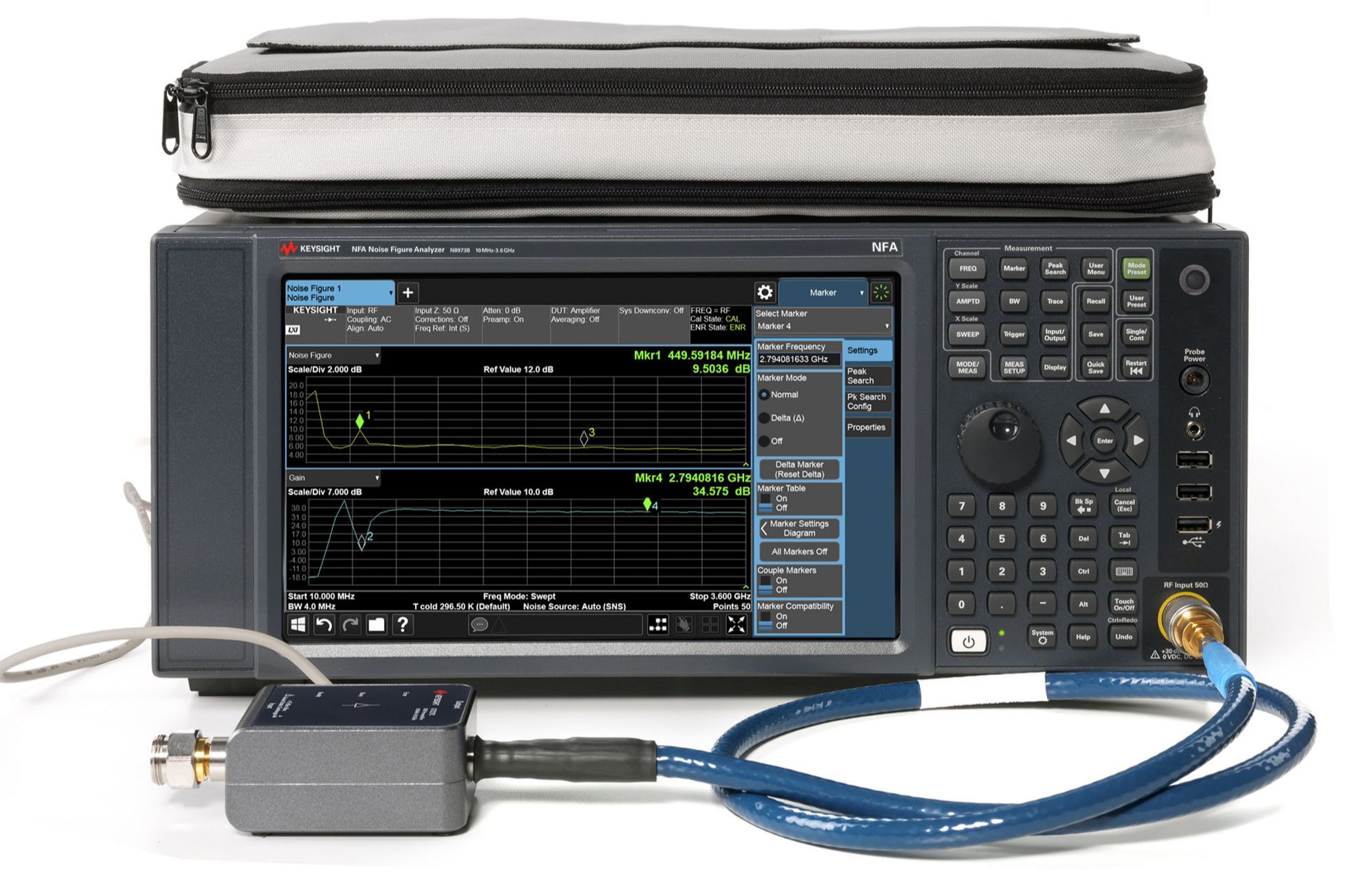
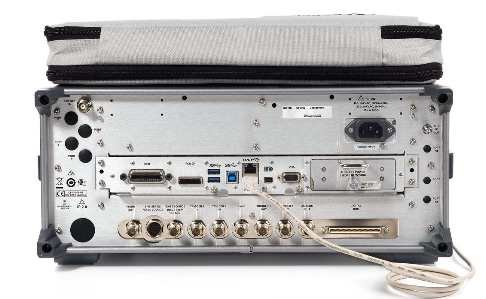
NFA X系列N8973B 510 MHz 至 3.6 GHz噪声系数分析仪,多点触控|是德/KEYSIGHT (在产)
参考价格 : USD 72,394.39至USD 78,951.39
产品描述
详细指标
软件和手册|白皮书
购买渠道
选件
问大家
视频
测评
口碑
系统与解决方案
是德科技|KEYSIGHT
NF7 系列噪声系数分析仪,10 MHz 至 3.6 GHz,多点触控
快速、精确的噪声系数测量
产品简介
综合解决方案提供 10 MHz 至 3.6 GHz 的频率范围多点触控界面包括频谱分析仪和 IQ 分析仪(基础)模式内置标配选件包括 P03、PFR、FSA、
NFE 和 B25 N型(阴头)输入连接器与 SNS 系列噪声源兼容:N4000A 、N4001A 、N4002A 包括 U7227A 10 MHz
核心参数
• 增益不确定度:±0.15 dB
• 带宽:8 MHz
• 最高频率:3.6 GHz
• 仪器不确定度:±0.02 dB(使用 4-6 dB ENR 噪声源)
功能特性
• 产品亮点
综合解决方案提供 10 MHz 至 3.6 GHz 的频率范围
多点触控界面
包括频谱分析仪和 IQ 分析仪(基础)模式
内置标配选件包括 P03、PFR、FSA、NFE 和 B25
N型(阴头)输入连接器
与 SNS 系列噪声源兼容:N4000A 、N4001A 、N4002A
包括 U7227A 10 MHz 至 4 GHz 外部 USB 前置放大器
N8973B 高性能噪声系数分析仪可进行快速、准确且可重复的噪声系数测量。
当与 SNS 系列噪声源和 U7227 系列 USB 前置放大器配合使用时,
来自 SNS 的 ENR 数据和 USB 前置放大器数据会自动下载至 N8973B。
N8973B 配备多点触控界面,支持放大、缩小和拖动手势。
只需轻点指尖,即可访问多数菜单,无需切换屏幕。
通过一步完成多达12种被测器件设置的综合校准,显著简化了Y因子测量中的噪声源校准。
利用内部校准功能,无需执行用户校准,可为多种类型的被测器件节省宝贵的测试时间。
内置噪声系数不确定度计算器可预先填入来自 SNS 噪声源、USB 前置放大器的数据,以及所有必要的仪器参数,
例如分析仪噪声系数、增益、噪声系数不确定度以及匹配等。
默认噪声系数设置提供了同时的噪声系数和增益测量。
使用表格(Table)视图,可以以表格形式同时查看多种测量结果,包括噪声系数、噪声因数、Y 因数、增益、Phot 、
Pcold 和 Teffective 。
N8973B 的频谱分析仪模式和 IQ 分析仪(基础)模式提供了额外的灵活性,使客户除了能够测量噪声系数之外,
还能根据需要更深入地分析被测器件特性。
3 GHz 内置前置放大器(选件 P03)、25 MHz 分析带宽(选件 B25)、精密频率参考(选件 PFR)、
精细步进衰减器(选件 FSA)和本底噪声扩展(选件 NFE)作为标准选件提供。
此外,随附的卡扣式附件袋可容纳外部 USB 前置放大器、噪声源和适配器。
通过以太网、USB 或 GPIB 接口连接至是德科技信号发生器,可实现外部模拟本振与频率转换器件输入的连接。
本振控制可通过 N8973B 进行调整。
资源下载
以上内容与指标均取自是德科技(KEYSIGHT)官网该产品详情页与官方产品资料,未标注口径的为厂家公布值。
是德科技|KEYSIGHT · onetest 仪器资源库
是德科技 | KEYSIGHT
NFA X系列N8973B 510 MHz 至 3.6 GHz噪声系数分析仪,多点触控 详细指标
快速、精确的噪声系数测量
一、通用规格
说明规格补充信息
条件:computed by the uncertainty calculator. Also, there is a paucity of available noise sources in this range.
Noise Figure Uncertainty Calculatora a. To compute the total uncertainty for your noise figure measurement, you need to take into account other fac- tors including: DUT NF, Gain and Match, Instrument NF, Gain Uncertainty and Match; Noise source ENR uncer- tainty and Match. The computations can be performed with the uncertainty calculator included with the Noise
Figure Measurement Personality. Go to Mode Setup then select Uncertainty Calculator. Similar calculators are
<10 MHz See noteb
b. Instrument Uncertainty is nominally the same in this frequency range as in the higher frequency range. How-
ever, total uncertainty is higher because the analyzer has poorer noise figure, leading to higher uncertainties as
10 MHz to internal preamplifier’s
条件:that depends on the Y factor to give the total uncertainty of the noise figure or gain measurement.
See Keysight App Note 57-2, literature number 5952-3706E for details on the use of this specification.
est bandwidth with uncompromised accuracy. e. The instrument uncertainties shown are under best-case sw eep time conditions, which is a sweep time near to the period of the power line, such as 20 ms for 50 Hz power sources. The behavior can be greatly degraded (uncertainty increased nominally by 0.12 dB) by setting the sweep time per point far from an integer multiple of
Uncertaintyde d. “Instrument Uncertainty” is defined for noise figure analysis as uncertainty due to relative amplitude uncertain- ties encountered in the analyzer when making the measurements required for a noise figure computation. The relative amplitude uncertainty depends on, but is not identical to, the relative display scale fidelity, also known
as incremental log fidelity. The uncertainty of the analyzer is multiplied within the computation by an amount
Jitter (amplitude variations) will also affect the accuracy of results. The standard deviation of the measured
result decreases by a factor of the square root of the Resolution Bandwidth used and by the square root of the
number of averages. This application uses the
4 MHz Resolution Bandwidth as default because this is the wid-
the period of the line frequency. 4 to 6.5 dB 0 to 20 dB ±0.02 dB 12 to 17 dB 0 to 30 dB ±0.025 dB 20 to 22 dB 0 to 35 dB
±0.03 dB
二、通用规格
条件:ties encountered in the analyzer when making the measurements required for the gain computation.
See Keysight App Note 57-2, literature number 5952-3706E for details on the use of this specification.
Instrument Uncertaintya DUT Gain Range =
−20 to +40 dB
<10 MHz See noteb
10 MHz to 3.6 GHz
±0.15 dB
>3.6 GHz ±0.11 dB additionalc
95th percentile
5 minutes after calibration
a. “Instrument Uncertainty” is defined for gain measuremen ts as uncertainty due to relative amplitude uncertain-
Jitter (amplitude variations) will also affect the accuracy of results. The standard deviation of the measured
result decreases by a factor of the square root of the Resolution Bandwidth used and by the square root of the
number of averages. This application uses the
4 MHz Resolution Bandwidth as default since this is the widest
带宽(含) uncompromised 精度
条件:Under difficult conditions (low Y factors), the instrument uncertainty for gain in high band can dominate the NF
impacting gain directly. When the Y factor is large, the effect of IU of Gain on the NF becomes negligible.
of the IU for NF for 4 − 6.5 dB ENR sources and the shown “additional” IU for gain for this frequency range.
sum of IU for Gain in the 0.01 − 3.6 GHz range and the “additional” IU shown.
uncertainty as well as causing errors in the measurement of gain. These effects can be predicted with the
uncertainty calculator. b. Uncertainty performance of the instrument is nominally the same in this frequency range as in the higher fre- quency range. However, performance is not warranted in this range. There is a paucity of available noise sources in this range, and the analyzer has poorer noise figure, leading to higher uncertainties as computed by
the uncertainty calculator. c. For frequencies above
3.6 GHz, the analyzer uses a YIG- tuned filter (YTF) as a preselector, which adds uncer- tainty to the gain. When the Y factor is small, such as with low gain DUTs, this uncertainty can be greatly multi- plied and dominate the uncertainty in NF (as the user can compute with the Uncertainty Calculator), as well as
When the Y-factor is small, the non-YTF mechanism that causes Instrument Uncertainty for Gain is the same as
the one that causes IU for NF with low ENR. Therefore, we would recommend the following practice: When
using the Uncertainty Calculator for measurements above
3.6 GHz, fill in the IU for Gain parameter with the sum
When estimating the IU for Gain for the purposes of a gain measurement for frequencies above
3.6 GHz, use the
You will find, when using the Uncertainty Calculator, that the IU for Gain is only important when the input noise
of the spectrum analyzer is significant compared to the output noise of the DUT. That means that the best
devices, those with high enough gain, will have comparable uncertainties for frequencies below and above
3.6 GHz.
The additional uncertainty shown is that observed to be met in 95% of the frequency/instrument combinations
tested with 95% confidence. It is not warranted.
三、通用规格
噪声 Figure 不确定度 Calculatora
条件:Instrument Noise Figure See graphs of “Nominal Instrument Noise
Instrument Noise Figure Uncertainty See the Noise Figure table earlier in this chapter
Instrument Gain Uncertainty See the Gain table earlier in this chapter
Figure”; Noise Figure is DANL +
176.24 dB
Note on DC couplingc
Optional NFE Improvement/Internal Cale See “Displayed Average Noise Level
(DANL) ((含) 噪声底 Extension)
条件:Option NFE - Noise Floor Extension chapter. a. The Noise Figure Uncertainty Calculator requires the para meters shown in order to calculate the total uncertainty of a Noise Figure measurement.
Improvement” on page
89 in the
b. Nominally, the noise figure of the spectrum analyzer is given by
NF = D − (K − L + N + B) where D is the DANL (displayed average noise level) specification,
K is kTB (−173.98 dBm in a
1 Hz bandwidth at 290 K)
L is
2.51 dB (the effect of log averaging used in DANL verifications)
N is
0.24 dB (the ratio of the noise bandwidth of the RBW filter with which DANL is
specified 至 ideal 噪声带宽)
条件:The actual NF will vary from the nominal due to frequency response errors.
mended for the best measurements. d. The instrument NF nominally degrades by 0.2 dB at 30 MHz and 1 dB at 10 MHz with AC coupling. e. With Option NFE (Noise Floor Extension) use that capability in the Noise Figure Measurement Application to allow "Internal Cal" instead of user calibration. With internal calibration, the measurement is much better than an
B is ten times the base-10 logarithm of the RBW (in hertz) in which the DANL is
specified. B is 0 dB for the
1 Hz RBW.
c. The effect of AC coupling is negligible for frequenc ies above 40 MHz. Below
40 MHz, DC coupling is recom-
uncalibrated measurement but not as good as with user calibration. Calibration reduces the effect of the analyzer
noise on the total measured NF. With user calibration, the extent of this reduction is computed in the uncertainty
calculator, and will be on the order of 16 dB. With internal calibration, the extent of reduction of the effective
noise level varies with operating frequency, its statistics are given on the indicated page. It is usually about half as
effective as User Calibration, and much more convenient. For those measurement situations where the output
noise of the DUT is
10 dB or more above the instrument input noise, the errors due to using an internal calibration
四、通用规格
校准选件
条件:Internal Calibration Good uncertainties without the n eed of reconnecting the DUT and running a calibration.
Nominal Instrument Noise Figure, N8973B-N8976B [Plot]
User Calibration Best uncertainties; Noise Figure Uncertainty Calculator applies
Uncalibrated Worst uncertainties; noise of the analyzer input acts as a second stage noise on the DUT
The uncertainty of the analyzer input noise model adds a second-stage noise power to
the DUT that can be positive or negative. Running the Noise Figure Uncertainty
Calculator will usually show that internal Calibration achieves
90% of the possible
improvement between the Uncalibrated and User Calibration states.
五、通用规格
适用型号 N8973B-N8976B
Specification Guide
2 NFA X-Series Noise Figure Analyzer - SA Mode
This chapter contains the specifications for the core analyzer. The
specifications and characteristics for the measurement applications and
术语定义和要求
条件:nominal values are described as follows.
This book contains signal analyzer specifications and supplemental
information. The distinction among specifications, typical performance, and
条件:temperature range" or "Full range", unless otherwise noted).
— Specifications describe the performance of parameters covered by the
product warranty (temperature =
0 to 55°C also referred to as "Full
— 95th percentile values indicate the breadth of the population (≈2σ) of
performance tolerances expected to be met in 95% of the cases with a
95%
confidence, for any ambient temperature in the range of 20 to 30°C. In
addition to the statistical observations of a sample of instruments, these
values include the effects of the uncertainties of external calibration
references. These values are not warranted. These values are updated
occasionally if a significant change in the statistically observed behavior of
production instruments is observed
— Typical describes additional product performance information that is not
covered by the product warranty. It is performance beyond specification
that 80% of the units exhibit with a
95% confidence level over the
temperature range
20 to 30°C. Typical performance does not include
测量不确定度
条件:— Nominal values indicate expected performance, or describe product
performance that is useful in the application of the product, but is not
六、条件 Required 至 Meet 规格
— The analyzer is within its calibration cycle. See the General section of this
— Under auto couple control, except that Auto Sweep Time Rules = Accy.
— For signal frequencies <
10 MHz, DC coupling applied.
— Any analyzer that has been stored at a temperature range inside the
allowed storage range but outside the allowed operating range must be
stored at an ambient temperature within the allowed operating range for at
least two hours before being turned on
条件:run recently enough to prevent an Alert message. If the Alert condition is
— The analyzer has been turned on at least
30 minutes with Auto Align set to
Normal, or if Auto Align is set to Off or Partial, alignments must have been
changed from “Time and Temperature” to one of the disabled duration
NFA X-Series 噪声 Figure 分析仪 - SA 模式
条件:Definitions and Requirements choices, the analyzer may fail to meet specifications without informing the user. If Auto Align is set to Light, performance is not warranted, and nominal performance will degrade to become a factor of 1.4 wider for any
specification subject to alignment, such as amplitude tolerances
Keysight Technologies certifies that this product met its published
specifications at the time of shipment from the factory. Keysight Technologies
further certifies that its calibration measurements are traceable to the United
States National Institute of Standards and Technology, to the extent allowed
by the Institute’s calibration facility, and to the calibration facilities of other
最大值频率
N8973B
3.6 GHz
N8974B
7 GHz
N8975B
26.5 GHz
N8976B
44 GHz
Preamp Option P03
3.6 GHz
Preamp Option P07
7 GHz
Preamp Option P26
26.5 GHz
Preamp Option P44
44 GHz
DC Coupled
Off 10 MHz
10 Hz
On 10 MHz
100 kHz
Mixing Mode
LO Multiple (Nb) Band Overlaps c 0 (10 Hz to 3.6 GHz) 1 − 1 N8973B-N8976B 1 (3.5 GHz to 7 GHz) 1 − 1 N8974B 1 (3.5 GHz to 8.4 GHz) 1 −
1 N8975 and N8976B
2 (8.3 GHz to 13.6 GHz) 1 −
2 N8974B, N8975B, and N8976B
3 (13.5 to 17.1 GHz) 2 −
2 N8975B and N8976B
4 (17.0 to 26.5 GHz) 2 −
4 N8975B and N8976B
5 (26.4 GHz to 34.5 GHz) 2 −
4 N8976B
6 (34.4 GHz to 44 GHz) 4 −
8 N8976B
NFA X-Series 噪声 Figure 分析仪 - SA 模式
条件:described as “3.5 to 7.0 GHz” represent nominal performance from 3.5 to 3.6 GHz, and warranted performance
Frequency and Time b. N is the LO multiplication factor. For ne gative mixing modes (as indicated by the “−” in the “Harmonic Mixing
Mode” column), the desired 1st LO harmonic is higher than the tuned frequency by the
1st IF (5.1225 GHz for
band 0
322.5 MHz for all other bands).
c. In the band overlap regions, for exam ple
3.5 to 3.6 GHz, the analyzer may use either band for measurements, in
this example Band 0 or Band 1. The analyzer gives preference to the band with the better overall specifications
(which is the lower numbered band for all frequencies below
26 GHz), but will choose the other band if doing so is
necessary to achieve a sweep having minimum band crossings. For example, with CF =
3.58 GHz, with a span of
40 MHz or less, the analyzer uses Band 0, because the stop frequency is
3.6 GHz or less, allowing a span without
band crossings in the preferred band. If the span is between 40 and 160 MHz, the analyzer uses Band
1, because
the start frequency is above 3.5 GHz, allowing the sweep to be done without a band crossing in Band
1, though
the stop frequency is above 3.6 GHz, preventing a Band
0 sweep without band crossing. With a span greater than
160 MHz, a band crossing will be required: the analyzer sweeps up to 3.6 GHz in Band
0; then executes a band
crossing and continues the sweep in Band
1.
Specifications are given separately for each band in the band overlap regions. One of these specifications is for the
preferred band, and one for the alternate band. Continuing with the example from the previous paragraph
(3.58 GHz), the preferred band is band 0 (indicated as frequencies under
3.6 GHz) and the alternate band is band
1 (3.5 to 8.4 GHz). The specifications for the preferred band are warranted. The specifications for the alternate
band are not warranted in the band overlap region, but performance is nominally the same as those warranted
specifications in the rest of the band. Again, in this example, consider a signal at 3.58 GHz. If the sweep has been
configured so that the signal at 3.58 GHz is measured in Band 1, the analysis behavior is nominally as stated in the
Band
1 specification line (3.5 to 8.4 GHz) but is not warranted. If warranted performance is necessary for this sig-
nal, the sweep should be reconfigured so that analysis occurs in Band
0. Another way to express this situation in
this example Band 0/Band 1 crossing is this: The specifications given in the “Specifications” column which are
from 3.6 to 7.0 GHz.
Precision 频率参考 (选件 PFR 标配)
条件:Aging Rate ±5 × 10⁻¹⁰/day (nominal)
Warm-up and Retraced Nominal 300 s after turn on ±1 × 10⁻⁷ of final frequency 900 s after turn on ±1 × 10⁻⁸ of final frequency
Accuracy ±[(time since last adjustment × aging rate) + temperature stability + calibration accuracya]b
Temperature Stability 20 to 30°C ±1.5 ×
10−8 Nominally linearc
Full temperature range ±5 ×
10−8
Total Aging 1 Year ±1 × 10⁻⁷ 2 Years ±1.5 ×
10−7
Settability ±2 ×
10−9
Achievable Initial Calibration Accuracye ±4 ×
10−8
Standby power to reference oscillator Not supplied
条件:(nominal) a. Calibration accuracy depends on how accurately the frequency standard was adjusted to 10 MHz. If the adjust- ment procedure is followed, the calibration accuracy is given by the specification “Achievable Initial Calibration
Accuracy.” b. The specification applies after the analyzer has been powered on for four hours. c. Narrow temperature range performance is nomina lly linear with temperature. For example, for 25±3º C, the stability would be only three-fifths as large as the warranted 25±5º C, thus ±0.9 × 10⁻⁸.
Residual FM (Center Frequency = 1 GHz 10 Hz RBW
10 Hz VBW)
≤0.25 Hz × Nf p-p in 20 ms
d. Standby mode does not apply power to the oscillator . Therefore warm-up applies every time the power is
turned on. The warm-up reference is one hour after turning the power on. Retracing also occurs every time
warm-up occurs. The effect of retracing is included within the “Achievable Initial Calibration Accuracy” term of
NFA X-Series 噪声 Figure 分析仪 - SA 模式
Frequency and Time e. The achievable calibration accuracy at the beginning of the calibration cycle includes these effects: 1) Temperature difference between the calibration environment and the use environment 2) Orientation relative to the gravitation field changing between the calibration environment and the use envi-
ronment 3) Retrace effects in both the calibration environment and the use environment due to turning the instrument power off.
4) Settability
说明规格补充信息
Frequency Readout Accuracy ±(marker freq × freq ref accy. +
0.25% ×
span + 5% × RBWa + 2 Hz +
0.5 × horizontal
Single detector onlyc
条件:Example for EMCd ±0.0032% (nominal)
a. The warranted performance is only the sum of all errors under autocoupled conditions. Under non-autocoupled
conditions, the frequency readout accuracy will nominally meet the specification equation, except for conditions
in which the RBW term dominates, as explained in examples below. The nominal RBW contribution to frequency
widest autocoupled RBW), and 30% of RBW for the (manually selected) 4, 5, 6 and 8 MHz RBWs.
the total actual error (317 kHz) would still meet the computed specification (355 kHz).
autocoupled and there are 1001 sweep points, that exception occurs only for spans > 750 MHz.
c. Specifications apply to traces in most cases, but ther e are exceptions. Specifications always apply to the peak
detector. Specifications apply when only one detector is in use and all active traces are set to Clear Write. Spec-
points, the errors in excess of the bucket quantization limitation were negligible.
readout accuracy is 2% of RBW for RBWs from 1 Hz to 390 kHz, 4% of RBW from 430 kHz through
3 MHz (the
First example: a 120 MHz span, with autocoupled RBW. The autocoupled ratio of span to RBW is
106:1, so
the RBW selected is 1.1 MHz. The 5% × RBW term contributes only
55 kHz to the total frequency readout accu-
racy, compared to 300 kHz for the
0.0.25% × span term, for a total of 355 kHz. In this example, if an instrument
had an unusually high RBW centering error of 7% of RBW (77 kHz) and a span error of 0.20% of span (240 kHz),
Second example: a 20 MHz span, with a
4 MHz RBW. The specification equation does not apply because the
Span: RBW ratio is not autocoupled. If the equation did apply, it would allow
50 kHz of error (0.25%) due to the
span and 200 kHz error (5%) due to the RBW. For this non-autocoupled RBW, the RBW error is nominally
30%
or 1200 kHz.
b. Horizontal resolution is due to the marker readin g out one of the sweep points. The points are spaced by
span/(Npts –1), where Npts is the number of sweep points. For example, with the factory preset value of 1001
sweep points, the horizontal resolution is span/1000. However, there is an exception: When both the detector
mode is “normal” and the span > 0.25 × (Npts –1) × RBW, peaks can occur only in even-numbered points, so
the effective horizontal resolution becomes doubled, or span/500 for the factory preset case. When the RBW is
ifications also apply when only one detector is in use in all active traces and the "Restart" key has been pressed
since any change from the use of multiple detectors to a single detector. In other cases, such as when multiple
simultaneous detectors are in use, additional errors of 0.5
1.0 or 1.5 sweep points will occur in some detectors
depending on the combination of detectors in use. d. In most cases, the frequency readout accuracy of the an alyzer can be exceptionally good. As an example, Key- sight has characterized the accuracy of a span commonly used for Electro-Magnetic Compatibility (EMC) testing using a source frequency locked to the analyzer. Ideally, this sweep would include EMC bands C and D and thus
sweep from 30 to 1000 MHz. Ideally, the analysis bandwidth would be
120 kHz at −6 dB, and the spacing of the
points would be half of this (60 kHz). With a start frequency of 30 MHz and a stop frequency of 1000.2 MHz and
a total of 16168 points, the spacing of points is ideal. The detector used was the Peak detector. The accuracy of
frequency readout of all the points tested in this span was with ±0.0032% of the span. A perfect analyzer with
this many points would have an accuracy of ±0.0031% of span. Thus, even with this large number of display
Frequency Countera See noteb
条件:a. Instrument conditions: RBW = 1 kHz, gate time = auto (100 ms), S/N ≥ 50 dB, frequency = 1 GHz
accuracy is ±0.100 Hz under the test conditions of footnote a. This error is a noisiness of the result. It will
increase with noisy sources, wider RBWs, lower S/N ratios, and source frequencies > 1 GHz.
Count Accuracy ±(marker freq × freq ref accy. +
0.100 Hz)
Delta Count Accuracy ±(delta freq. × freq ref accy. +
0.141 Hz)
Resolution
0.001 Hz
b. If the signal being measured is locked to the same frequency reference as the analyzer, the specified count
N8973B 0 Hz
10 Hz to 3.6 GHz
N8974B 0 Hz
10 Hz to 7 GHz
N8975B 0 Hz
10 Hz to 26.5 GHz
N8976B 0 Hz
10 Hz to 44 GHz
Resolution
2 Hz
跨度精度
条件:auto coupled and there are 1001 sweep points, that exception occurs only for spans > 750 MHz.
Swept ±(0.25% × span + horizontal resolutiona)
FFT ±(0.1% × span + horizontal resolutiona)
a. Horizontal resolution is due to the marker reading out one of the sweep points. The points are spaced by
span/(Npts − 1), where Npts is the number of sweep points. For example, with the factory preset value of 1001
sweep points, the horizontal resolution is span/1000. However, there is an exception: When both the detector
mode is “normal” and the span > 0.25 × (Npts − 1) × RBW, peaks can occur only in even-numbered points, so
the effective horizontal resolution becomes doubled, or span/500 for the factory preset case. When the RBW is
扫描时间范围
Span =
0 Hz
Span ≥
10 Hz
1 μs to 6000 s
1 ms to 4000 s
扫描时间精度
Span ≥
10 Hz, swept
Span ≥
10 Hz, FFT
Span =
0 Hz
±0.01% (nominal)
±40% (nominal)
±0.01% (nominal)
Sweep Trigger Free Run, Line, Video, External
1
External
2, RF Burst, Periodic Timer
条件:a. Delayed trigger is available with line, video, RF burst and external triggers.
Span ≥ 10 Hz, swept
0 to 500 ms
Span = 0 Hz or FFT
−150 ms to +500 ms
Resolution
0.1 μs
Additional information on some of the triggers and gate sources
Video Independent of Display Scaling and Reference Level
条件:Maximum usable level Highest allowed mixer level a + 2 dB (nominal)
Minimum settable level
−170 dBm Useful range limited by noise
Negative Peak
Triggers on the signal before detection, which is similar to the displayed signal
检波器 = Average
Triggers on the signal before detection, but with a single-pole filter added to give similar smoothing to that of the average detector
扫描类型 = FFT
Triggers on the signal envelope in a bandwidth wider than the FFT width
LO feedthrough can degrade or prevent triggering
How close is too close depends on the bandwidth listed above.
External Triggers See “Trigger Inputs” on page
68
幅度要求
–65 dBm minimum video carrier power at the input
NTSC-4.43,
PAL-60, SECAM-L
One, Field Two
Line Selection
1 to 525, or 1 to 625
NFA X-Series 噪声 Figure 分析仪 - SA 模式
条件:Low. b. Noise will limit trigger level range at high frequencies, such as above 15 GHz.
Frequency and Time a. The highest allowed mixer level depends on the IF Gain. It is nominally
–10 dBm for Preamp Off and IF Gain =
跨度范围 Any 跨度
条件:Gate Delay Jitter 33.3 ns p-p (nominal)
Gate Length Range (Except Method = FFT) 100 ns to 5.0 s Gate length for the FFT method is fixed at 1.83/RBW, with nominally 2% tolerance.
Gate Delay Range
0 to 100.0 s
Gate Delay Settability 4 digits
≥100 ns
幅度误差
Nominally no additional error for gated measurements when the Gate Delay is greater than the MIN FAST setting
Gate Sources External
1
External
2
编号频率扫描 Points (buckets)
Factory preset
1001
Range
1 to 100,001 Zero and non-zero spans
分辨率带宽 (RBW)
Range (−3.01 dB bandwidth)
1 Hz to 8 MHz
Bandwidths above 3 MHz are 4, 5
6, and
8 MHz.
Bandwidths
1 Hz to 3 MHz are spaced at
10% spacing using the E24 series (24
per decade): 1.0, 1.1, 1.2, 1.3, 1.5
1.6
1.8, 2.0, 2.2, 2.4, 2.7, 3.0, 3.3, 3.6
3.9
4.3, 4.7, 5.1, 5.6, 6.2, 6.8, 7.5, 8.2
9.1 in
功率带宽 accuracya
条件:RBW Range CF Range 1 Hz to 750 kHz All ±1.0% (0.044 dB) 820 kHz to 1.2 MHz <3.6 GHz ±2.0% (0.088 dB) 1.3 to 2.0 MHz <3.6 GHz ±0.07 dB (nominal)
2.2 to 3 MHz <3.6 GHz 0 to −0.2 dB (nominal)
4 to 8 MHz <3.6 GHz 0 to −0.4 dB (nominal)
Noise BW to RBW ratiob 1.056 ±2% (nominal)
1 Hz to 1.3 MHz RBW ±2% (nominal)
Selectivity (−60 dB/−3 dB) 4.1:1 (nominal)
FFT Flattop. While the warranted performance only applies to the swept Gaussian filters, because only they are
kept under statistical process control, the other filters nominally have the same performance.
Accuracy (−3.01 dB bandwidth)c
1.5 MHz to 3 MHz RBW
CF ≤
3.6 GHz
CF >
3.6 GHz
±7% (nominal)
±8% (nominal)
4 MHz to 8 MHz RBW
CF ≤
3.6 GHz
CF >
3.6 GHz
±15% (nominal)
±20% (nominal)
a. The noise marker, band power marker, channel power a nd ACP all compute their results using the power band-
width of the RBW used for the measurement. Power bandwidth accuracy is the power uncertainty in the results
of these measurements due only to bandwidth-related errors. (The analyzer knows this power bandwidth for
each RBW with greater accuracy than the RBW width itself, and can therefore achieve lower errors.) The war-
ranted specifications shown apply to the Gaussian RBW filters used in swept and zero span analysis. There are
four different kinds of filters used in the spectrum analyzer: Swept Gaussian, Swept Flattop, FFT Gaussian and
NFA X-Series 噪声 Figure 分析仪 - SA 模式
条件:Frequency and Time b. The ratio of the noise bandwidth (also known as the power bandwidth) to the RBW has the nominal value and tolerance shown. The RBW can also be annotated by its noise bandwidth instead of this 3 dB bandwidth. The accuracy of this annotated value is similar to that shown in the power bandwidth
c. Resolution Bandwidth Accuracy can be observed at slow er sweep times than auto-coupled conditions. Normal
widening declines to 0.6% nominal when the Swp Time Rules key is set to Accuracy instead of Normal. The true
sweep rates cause the shape of the RBW filter displayed on the analyzer screen to widen by nominally
6%. This
bandwidth, which determines the response to impulsive signals and noise-like signals, is not affected by the
Analysis Bandwidtha
条件:nal can be digitized for further analysis or processing in the time, frequency, or modulation domain.
Standard
25 MHz
a. Analysis bandwidth is the instantane ous bandwidth available about a center frequency over which the input sig-
说明规格补充信息
条件:–3 dB Bandwidth –7.5% relative to –4 dB bandwidth, nominal
Preselector Bandwidth Relevant to many options, such as B25 Wide IF Bandwidth, in
Bands
1 and higher. Nominal.
Mean Bandwidth at CFa N8973B-N8975B N8976B
5 GHz 58 MHz
46 MHz
10 GHz 57 MHz
52 MHz
15 GHz 59 MHz
53 MHz
20 GHz 64 MHz
55 MHz
25 GHz 74 MHz
56 MHz
35 GHz
62 MHz
44 GHz
70 MHz
Standard Deviation 9%
7%
a. The preselector can have a signific ant passband ripple. To avoid ambiguous results, the
–4 dB bandwidth is
视频带宽 (VBW)
Range Same as Resolution Bandwidth range plus wide-open VBW (labeled
50 MHz)
Accuracy
±6% (nominal)
in swept mode and zero spana a. For FFT processing, the selected VBW is used to determine a number of averages for FFT results. That number is chosen to give roughly equivalent display smoothing to VBW filtering in a swept measurement. For example, if
VBW = 0.1 × RBW, four FFTs are averaged to generate one result.
测量范围
Preamp Off Displayed Average Noise Level to +23 dBm
Preamp On Displayed Average Noise Level to +23 dBm Option P03, P07, P26, P44
输入衰减范围
条件:With Option FSA (standard) 0 to 60 dB, in 2 dB steps
Standard
0 to 60 dB, in 10 dB steps
说明规格补充信息
Maximum Safe Input Level Applies with or without preamp (Option P03, P07, P26, P44)
Average Total Power
+30 dBm (1 W)
Peak Pulse Power (≤10 μs pulse width,
≤1% duty cycle,
input attenuation ≥
30 dB)
+50 dBm (100 W)
DC voltage
DC Coupled
±0.2 Vdc
AC Coupled
±100 Vdc
显示范围
Log Scale Ten divisions displayed
0.1 to 1.0 dB/division in 0.1 dB steps, and 1 to 20 dB/division in 1 dB steps
Log (decibel) units
条件:Linear units resolution ≤1% of signal level (nominal)
Trace Averaging Off, on-screen
0.01 dB
Trace Averaging On or remote
0.001 dB
频率响应参见 footnote
条件:ifications. (Maximum error relative to reference condition (50 MHz)
Band Overlaps on page
18.
Freq Option
526 only: Modes
above
18 GHza
a. Signal frequencies between
18 and 26.5 GHz are prone to additional response errors due to modes in the Type-N
connector used with Model N8975B. With the use of Type-N to APC 3.5 mm adapter part number
1250-1744
there are nominally six such modes. The effect of these modes with this connector are included within these spec-
Swept operationb
Attenuation
10 dB)
适用型号 N8976B (mmW)
N8973B-N8975B(RF/μW)
20 to 30°C Full range
95 th Percentile (≈2σ)
9 kHz to 10 MHz x ±0.8 dB ±1.0 dB
±0.40 dB
9 kHz to 10 MHz x ±0.6 dB ±0.8 dB
±0.28 dB
10 MHzc to 3.6 GHz x ±0.6 dB ±0.65 dB
±0.21 dB
10 to 50 MHz x ±0.45 dB ±0.57 dB
±0.21 dB
50 MHz to 3.6 GHz x ±0.45 dB ±0.70 dB
±0.20 dB
3.5 to 7 GHzde x ±2.0 dB ±3.0 dB
±0.69 dB
3.5 to 5.2 GHzde x ±1.7 dB ±3.5 dB
±0.91 dB
5.2 to 8.4 GHzde x ±1.5 dB ±2.7 dB
±0.61 dB
7 to 13.6 GHz x ±2.5 dB
±3.2 dB
8.3 to 13.6 GHzde x ±2.0 dB ±2.7 dB
±0.61 dB
13.5 to 22 GHzde x ±3.0 dB
±3.7 dB
13.5 to 17.1 GHzde x ±2.0 dB ±2.7 dB
±0.67 dB
17.0 to 22 GHzde x ±2.0 dB ±3.0 dB
±0.78 dB
22.0 to 26.5 GHzde x ±3.2 dB
±4.2 dB
22.0 to 26.5 GHzde x ±2.5 dB ±3.5 dB
±0.72 dB
26.4 to 34.5 GHzde x ±2.5 dB ±3.5 dB
±1.11 dB
34.4 to 44 GHzde x ±3.2 dB ±4.9 dB
±1.42 dB
NFA X-Series 噪声 Figure 分析仪 - SA 模式
条件:Amplitude Accuracy and Range b. For Sweep Type = FFT, add the RF flatness errors of this table to the IF Frequency Response errors. An additional error source, the error in switching between swept and FFT sweep types, is nominally ±0.01 dB and is included within the “Absolute Amplitude Error” specifications.
c. Specifications apply with DC coupling at all frequencies. With AC coupling, specifications apply at frequencies of
d. Specifications for frequencies > 3.5 GHz apply for sweep rates ≤100 MHz/ms.
50 MHz and higher. Statistical observations at 10 MHz show that most instruments meet the specifications, but a
few percent of instruments can be expected to have errors exceeding
0.5 dB at 10 MHz at the temperature
extreme. The effect at 20 to 50 MHz is negligible, but not warranted.
说明规格补充信息
IF Frequency Responsea Modes above
18 GHzb
(Demodulation and FFT response relative to the center frequency)
Preselector Max Errord (Exceptione)
Midwidth Error (95th
Slope (dB/MHz) (95th
RMSf (标称值)
条件:c. This column applies to the instantaneous analysis bandwid th in use. In the Spectrum Analyzer Mode, this would
MHz. f. The “rms” nominal performance is the standard deviation of the response relative to the center frequency, inte- grated across the span. This performance measure was observed at a center frequency in each harmonic mixing band, which is representative of all center frequencies; it is not the worst case frequency.
<3.6 ≤10 ±0.40 dB ±0.12 dB ±0.10
0.04 dB
≥3.6, ≤26.5 ≤10 On
0.25 dB
≥3.6 ≤10 Off ±0.45 dB ±0.12 dB ±0.10
0.04 dB
>26.5 ≤10 On
0.35 dB
a. The IF frequency response includes effects due to RF circuits such as input filters, that are a function of RF fre-
quency, in addition to the IF passband effects. b. Signal frequencies between 18 and 26.5 GHz are prone to additional response errors due to modes in the Type-N connector used with Model N8975B. With the use of Type-N to APC 3.5 mm adapter part number
1250-1744, there are nominally six such modes. These modes cause nominally up to −0.35 dB amplitude change, with phase
errors of nominally up to ±1.2°.
be the FFT width. d. The maximum error at an offset (f) from the cent er of the FFT width is given by the expression ± [Midwidth Error + (f × Slope)], but never exceeds ±Max Error. Here the Midwidth Error is the error at the center frequency for a given FFT span. Usually, the span is no larger than the FFT width in which case the center of the
FFT width is the center frequency of the analyzer. When using the Spectrum Analyzer mode with an analyzer span
is wider than the FFT width, the span is made up of multiple concatenated FFT results, and thus has multiple cen-
ters of FFT widths; in this case the f in the equation is the offset from the nearest center. Performance is nominally
three times better at most center frequencies. e. The specification does not apply for fr equencies greater than
3.6 MHz from the center in FFT widths of 7.2 to 8
IF 相位线性度 Deviation 从 mean 相位线性度
Modes above
18 GHza
RMS (标称值)b
条件:a linear phase condition, where the rms is computed across the span shown and over the range of center fre-
≥0.02, <3.6 ≤10 n/a 0.4°
0.1°
≥3.6, ≤10 Off 0.4°
0.1°
≥3.6 (Option ≤ 526) ≤10 On 1.0°
0.2°
a. Signal frequencies between
18 and 26.5 GHz are prone to additional response errors due to modes in the
Type-N connector used with Model N8975B. With the use Type-N to APC
3.5 mm adapter part number
1250-1744, there are nominally six such modes. These modes cause nominally up to −0.35 dB amplitude
change, with phase errors of nominally up to ±1.2°.
b. The listed performance is the standard deviation of the phase deviation relative to the mean phase deviation from
绝对幅度精度
条件:Amplitude Reference Accuracy ±0.05 dB (nominal)
(nominal) a. Absolute amplitude accuracy is the total of all ampl itude measurement errors, and applies over the following subset of settings and conditions: 1 Hz ≤ RBW ≤ 1 MHz; Input signal −10 to −50 dBm (details below); Input attenuation 10 dB; span < 5 MHz (nominal additional error for span ≥ 5 MHz is 0.02 dB); all settings auto-cou-
reduce noise. When using FFT sweeps, the signal must be at the center frequency.
the conditions listed above: Scale Fidelity, Reference Level Accuracy, Display Scale Switching Uncertainty, Res-
the instrument aligns its internal gains to the 50 MHz Amplitude Reference.
At 50 MHza
20 to 30°C
Full temperature range ±0.40 dB ±0.43 dB
±0.15 dB (95th percentile)
At all frequenciesa
20 to 30°C
Full temperature range ±(0.40 dB + frequency response) ±(0.43 dB + frequency response)
95th Percentile Absolute
Amplitude Accuracyb
±0.27 dB (Wide range of signal levels
RBWs, RLs, etc.
0.01 to 3.6 GHz
Atten =
10 dB)
Preamp Onc ±(0.39 dB + frequency response)
pled except Swp Time Rules = Accuracy; combinations of low signal level and wide RBW use VBW ≤
30 kHz to
This absolute amplitude accuracy specification includes the sum of the following individual specifications under
olution Bandwidth Switching Uncertainty
50 MHz Amplitude Reference Accuracy, and the accuracy with which
The only difference between signals within the range ending at –50 dBm and those signals below that level is
the scale fidelity. Our specifications show the possibility of increased errors below
–80 dBm at the mixer, thus
–70 dBm at the input. Therefore, one reasonably conservative approach to estimating the Absolute Amplitude
Uncertainty below –70 dBm at the mixer would be to ad d an additional
±0.10 dB (the difference between the
above
–80 dBm at the mixer scale fidelity at the lower level scale fidelity) to the Absolute Amplitude Uncer-
NFA X-Series 噪声 Figure 分析仪 - SA 模式
条件:Amplitude Accuracy and Range b. Absolute Amplitude Accuracy for a wide range of signal and measurement settings, covers the 95th percentile proportion with 95% confidence. Here are the details of what is covered and how the computation is made:
The wide range of conditions of RBW, signal level, VBW, reference level and display scale are discussed in foot-
worst of the two computed 95th percentile results (they ere very close) is shown.
note a. There are 44 quasi-random combinations used, tested at a
50 MHz signal frequency. We compute the
95th percentile proportion with 95% confidence for this set observed over a statistically significant number of
instruments. Also, the frequency response relative to the
50 MHz response is characterized by varying the signal
across a large number of quasi-random verification frequencies that are chosen to not correspond with the fre-
quency response adjustment frequencies. We again compute the
95th percentile proportion with 95% confi-
dence for this set observed over a statistically significant number of instruments. We also compute the
95th
percentile accuracy of tracing the calibration of the
50 MHz absolute amplitude accuracy to a national stan-
dards organization. We also compute the 95th percentile accuracy of tracing the calibration of the relative fre-
quency response to a national standards organization. We take the root-sum-square of these four independent
Gaussian parameters. To that rss we add the environmental effects of temperature variations across the
20 to
30°C range. These computations and measurements are made with the mechanical attenuator only in circuit,
set to the reference state of 10 dB.
A similar process is used for computing the result when using the electronic attenuator under a wide range of
settings: all even settings from 4 through
24 dB inclusive, with the mechanical attenuator set to 10 dB. Then the
c. Same settings as footnote a, except that the signal level at the preamp input is
−40 to −80 dBm. Total power at
preamp (dBm) = total power at input (dBm) minus input attenuation (dB). This specification applies for signal
frequencies above
100 kHz.
说明规格补充信息
条件:9 kHz to 3.6 GHz ±0.3 dB (nominal)
3.5 to 7.0 GHz ±0.5 dB (nominal)
7.0 to 13.6 GHz ±0.7 dB (nominal)
13.5 to 26.5 GHz ±0.7 dB (nominal)
26.5 to 44 GHz ±1.0 dB (nominal)
Input Attenuation Switching Uncertainty Refer to the footnote for
Band Overlaps on page
18
50 MHz (reference frequency) ±0.20 dB
±0.08 dB (typical)
Attenuation >
2 dB, preamp off
(Relative to 10 dB (reference setting))
说明规格补充信息
RF Input VSWR Nominala at tuned frequency, DC Coupled 10 dB attenuation, 50 MHz
1.07:1
输入衰减
Frequency 0 dB
≥10 dB
适用型号 N8973B-N8975B
10 MHz to 3.6 GHz <2.2:1
<1.2:1
3.6 to 26.5 GHz
<1.9:1
适用型号 N8976B
条件:Preselector Centering Open input a. The nominal SWR stated is at the worst case RF frequency in three representative instruments.
10 MHz to 3.6 GHz <2.2:1
<1.2:1
3.6 to 26.5 GHz
<1.5:1
26.5 to 44 GHz
<1.8:1
RF calibrator (e.g.
50 MHz) is On Open input
Alignments running Open input for so me, unless "All but RF" is selected
说明规格补充信息
Resolution Bandwidth Switching Uncertainty Relative to reference BW of 30 kHz,
verified in low banda 1.0 Hz to 3 MHz RBW
±0.10 dB
Manually selected wide RBWs: 4, 5, 6, 8 MHz
±1.0 dB
a. RBW switching uncertainty is verified at 50 MHz. It is consistent for all measurements made without the prese-
lector, thus in Band 0 and also in higher bands with the Preselector Bypass option. In preselected bands, the
slope of the preselector passband can interact with the RBW shape to make an apparent additional RBW
switching uncertainty of nominally
±0.05 dB/MHz times the RBW.
Log Units
−170 to +23 dBm, in 0.01 dB steps
Linear Units
707 pV to3.16 V, with 0.01 dB resolution (0.11%)
Accuracy
0 dBa
a. Because reference level affects only the display, not the measurement, it causes no additional error in measure-
显示刻度 Switching 不确定度
Switching between Linear and Log
0 dBa
Log Scale Switching
0 dBa
a. Because Log/Lin and Log Scale Switching affect only th e display, not the measurement, they cause no addi-
tional error in measurement results from trace data or markers.
显示刻度 Fidelityab
条件:Absolute Log-Linear Fidelity (Relative to the reference condition: −25 dBm input through 10 dB attenuation, thus
−35 dBm at the input mixer)
−80 dBm ≤ ML ≤ −10 dBm
±0.15 dB
ML < −80 dBm
±0.25 dB
Relative Fidelityd Applies for mixer levelc range from −10 to
−80 dBm, mechanical attenuator only,
前置放大器关, 和 dither 开
条件:Sum of the following terms: Nominal high level term Up to ±0.045 dBe instability term Up to ±0.018 dB slope term From equationf
due to noise can be estimated from the equation below, given for the 3-sigma (three standard deviations) level.
level signals, around −60 dBm or lower, will nominally degrade by 0.2 dB.
c. Mixer level = Input Level − Input Attenuation d. The relative fidelity is the error in the measured difference between two signal levels. It is so small in many cases that it cannot be verified without being dominated by measurement uncertainty of the verification. Because of this verification difficulty, this specification gives nominal performance, based on numbers that are as conserva-
equation to compute the nominal performance.
prefilter term Up to ±0.005 dBg
a. Supplemental information: The amplitude detection linearity specification applies at all levels below
−10 dBm at
the input mixer; however, noise will reduce the accuracy of low level measurements. The amplitude error due to
noise is determined by the signal-to-noise ratio, S/N. If the S/N is large (20 dB or better), the amplitude error
The errors due to S/N ratio can be further reduced by averaging results. For large S/N (20 dB or better), the
3-sigma level can be reduced proportional to the square root of the number of averages taken.
b. The scale fidelity is warranted with ADC dither set to Medium. Dither increases the noise level by nominally only
0.1 dB for the most sensitive case (preamp Off, best DANL frequencies). With dither Off, scale fidelity for low
tively determined as those used in warranted specifications. We will consider one example of the use of the error
Example: the accuracy of the relative level of a sideband around
−60 dBm, with a carrier at −5 dBm, using atten-
uation = 10 dB, RBW =
3 kHz, evaluated with swept analysis. The high level term is evaluated with P1 =
−15 dBm and P2 = −70 dBm at the mixer. This gives a maximum error within
±0.025 dB. The instability term is
±0.018 dB. The slope term evaluates to ±0.050 dB. The prefilter term applies and evaluates to the limit of
±0.005 dB. The sum of all these terms is
±0.098 dB.
3σ 32 0dB() 11 0 SN⁄ 3dB+()
20dB⁄()–+log=
NFA X-Series 噪声 Figure 分析仪 - SA 模式
条件:the highest power for which linearity is specified). All these levels are referred to the mixer level.
f. Slope error will nominally be well within the range of ±0.0009 × (P1 − P2). P1 and P2 are defined in footnote e.
Amplitude Accuracy and Range e. Errors at high mixer levels will nominally be well within the range of ±0.045 dB × {exp[(P1 − Pref)/(8.69 dB)] − exp[(P2 − Pref)/(8.69 dB)]} (exp is the natural exponent function, e x). In this expression, P1 and P2 are the pow- ers of the two signals, in decibel units, whose relative power is being measured. Pref is
−10 dBm (−10 dBm is
g. A small additional error is possible. In FFT sweeps, th is error is possible for spans under
4.01 kHz. For non-FFT
measurements, it is possible for RBWs of 3.9 kHz or less. The error is well within the range of ±0.0021 × (P1 -
P2) subject to a maximum of ±0.005 dB. (The maximum dominates for all but very small differences.) P1 and P2
增益压缩
Description Specifications Supplemental Information
1 dB Gain Compression Point (Two-tone)abc a. Large signals, even at frequencies not shown on the screen, can cause the analyzer to incorrectly measur e on-scr
een signals because of two-tone gain compression. This specification tells how large an interfering signal
must be in order to cause a
1 dB change in an on-screen signal.
b. Specified at 1 kHz RBW with 100 kHz tone spacing. The compression point will nominally equal the specification
for tone spacing greater than
5 times the prefilter bandwidth. At smaller spacings, ADC clipping may occur at a
le vel lower than the
1 dB compression point. c. Reference level and off-screen performance: The referenc e level (RL) behavior differs from some earlier analyz- ers in a way that makes this analyzer more flexible. In other analyzers, the RL controlled how the measurement
was pe rformed as well as how it was displayed. Because the logarithmic amplifier in these analyzers had both range and resolution limitations, this behavior was necessary for optimum measurement accuracy. The logarith- mic amplifier in this signal analyzer, however, is implemented digitally such that the range and resolution greatly
exceed other instrument limitations. Because of this, the analyzer can make measurements largely independent
of the setting of the RL without compromising accuracy. Because the RL becomes a display function, not a mea- surement function, a marker can read out results that are off-screen, either above or below, without any change in accuracy. The only exception to the independence of RL and the way in which the measurement is performed
is in the input att enuation setting: When the input attenuation is set to auto, the rules for the determination of th e input attenuation include dependence on the reference level. Because the input attenuation setting controls
the tradeoff between large signal behaviors (third-order intermodulation, compression, and display scale fidel-
ity) and small signal effects (noise), the measurement results can change with RL changes when the input atten-
Clipping (ADC Over-range)
Any signal offset
−10 dBm Low frequency exceptionse
Signal offset >
5 times IF prefilter bandwidth and IF
Gain set to Low
+12 dBm (nominal)
IF Prefilter Bandwidth
Zero Span or Sweep Type = FFT
–3 dB Bandwidth
NFA X-Series 噪声 Figure 分析仪 - SA 模式
Dynamic Range e. The ADC clipping level declines at low frequencies (bel ow 50 MHz) when the LO feedthrough (the signal that appears at 0 Hz) is within 5 times the prefilter bandwidth (see table) and must be handled by the ADC. For
e xample, with a 300 kHz RBW and prefilter bandwidth at 966 kHz, the clipping level reduces for signal frequen- cies below 4.83 MHz. For signal frequencies below 2.5 times the prefilter bandwidth, there will be additional r
eduction due to the presence of the image signal (the signal that appears at the negative of the input signal fre-
Sample 或 Average 检波器
Averaging type = Log
0 dB input attenuation
IF Gain = High
1 Hz Resolution Bandwidth
Refer to the footnote for
Band Overlaps on page
18.
适用型号 N8976B (mmW)
条件:9 kHz to 1 MHz x –125 dBm (nominal)
N8973B-N8975B(RF/μW)
20 to 30°CF u l l r a n g e T y p i c a l
10 Hz x x
–90 dBm (nominal)
20 Hz x x
–100 dBm (nominal)
100 Hz x x
–110 dBm (nominal)
1 kHz x x
–120 dBm (nominal)
9 kHz to 1 MHz x
−130 dBm
1 to 10 MHzb x −147 dBm −145 dBm
−149 dBm
1 MHz to 1.2 GHz x −152 dBm −151 dBm
−155 dBm
10 MHz to 2.1 GHz x −148 dBm −146 dBm
−150 dBm
1.2 to 2.1 GHz x −151 dBm −150 dBm
−154 dBm
2.1 to 3.6 GHz x −147 dBm −145 dBm
−149 dBm
2.1 to 3.6 GHz x −149 dBm −148 dBm
−152 dBm
3.5 to 7 GHz x −147 dBm −145 dBm
−149 dBm
3.5 to 4.2 GHz x −144 dBm −142 dBm
−147 dBm
4.2 to 8.4 GHz x −145 dBm −143 dBm
−150 dBm
7 to 13.6 GHz x −143 dBm −141 dBm
−147 dBm
8.3 to 13.6 GHz x −147 dBm −145 dBm
−150 dBm
13.5 to 20 GHz x −137 dBm −134 dBm
−142 dBm
13.5 to 20 GHz x −145 dBm −143 dBm
−148 dBm
NFA X-Series 噪声 Figure 分析仪 - SA 模式
条件:Additional DANL, IF Gain=Lowc x x −160.5 dBm (nominal)
because the noise figure does not depend on RBW and 1 kHz measurements are faster.
b. DANL below 10 MHz is affected by phase noise around th e LO feedthrough signal. Specifications apply with the
cies below 25 kHz, and “Best Wide Offset φ Noise" for frequencies above 25 kHz.
coupling or manual coupling, there is noise added above that specified in this table for the IF Gain = High case.
Dynamic Range 20 to 26.5 GHz x −134 dBm −130 dBm −140 dBm 20 to 26.5 GHz x −142 dBm −140 dBm −145 dBm 26.4 to 34 GHz x −140 dBm −136 dBm
−144 dBm
33.9 to 44 GHz x −135 dBm −131 dBm
−140 dBm
a. DANL for zero span and swept is measured in a 1 kH z RBW and normalized to the narrowest available RBW
best setting of the Phase Noise Optimization control, which is to choose the “Best Close-in φ Noise" for frequen-
c. Setting the IF Gain to Low is often desirable in order to allow higher power into the mixer without overload, bet-
ter compression and better third-order intermodulation. When the Swept IF Gain is set to Low, either by auto
That excess noise appears as an additional noise at the input mixer. This level has sub-decibel dependence on
center frequency. To find the total displayed average noise at the mixer for Swept IF Gain = Low, sum the powers
of the DANL for IF Gain = High with this additional DANL. To do that summation, compute DANLtotal =
10 × log
(10^(DANLhigh/10) + 10^(AdditionalDANL / 10)). In FFT sweeps, the same behavior occurs, except that FFT IF
Gain can be set to autorange, where it varies with the input signal level, in addition to forced High and Low set-
说明规格补充信息
Spurious Responses (see Band Overlaps on page
18)
前置放大器 Offa
Residual Responsesb
200 kHz to 8.4 GHz (swept)
Zero span or FFT or other frequencies
−100 dBm
−100 dBm (nominal)
Image Responses
Tuned Freq (f) Excitation Freq Mixer Levelc Response 10 MHz to 26.5 GHz f+45 MHz −10 dBm −75 dBc −99 dBc (typical) 10 MHz to 3.6 GHz f+10245 MHz −10 dBm −80 dBc −103 dBc (typical) 10 MHz to 3.6 GHz f+645 MHz −10 dBm −80 dBc
−107 dBc (typical)
3.5 to 13.6 GHz f+645 MHz −10 dBm −75 dBc
−87 dBc (typical)
13.5 to 17.1 GHz f+645 MHz −10 dBm −71 dBc
−85 dBc (typical)
17.0 to 22 GHz f+645 MHz −10 dBm −68 dBc
−82 dBc (typical)
22 to 26.5 GHz f+645 MHz −10 dBm −66 dBc
−78 dBc (typical)
26.5 to 34.5 GHz f+645 MHz −30 dBm –70 dBc
–94 dBc (typical)
34.4 to 44 GHz f+645 MHz −30 dBm –60 dBc
–79 dBc (typical)
Other Spurious Responses
Carrier Frequency
≤26.5 GHz
First RF Orderd (f ≥
10 MHz from carrier)
−10 dBm
−68 dBc +
20
Includes IF feedthrough, LO harmonic mixing responses
Higher RF Orderf (f ≥
10 MHz from carrier)
−40 dBm −80 dBc +
20
Includes higher order mixer responses
Carrier Frequency
>26.5 GHz
First RF Orderd (f ≥
10 MHz from carrier)
−30 dBm
–90 dBc (nominal)
Higher RF Orderf (f ≥
10 MHz from carrier)
−30 dBm
–90 dBc (nominal)
LO-Related Spurious Responses (f > 600 MHz from carrier
10 MHz to 3.6 GHz)
−10 dBm
−60 dBcg +
20 × log(Ne)
−90 dBc +
20 × log(N)
Sidebands, 偏置从 CW 信号
条件:200 Hz to 3 kHz −73 dBcg (nominal)
3 kHz to 30 kHz −73 dBc (nominal)
30 kHz to 10 MHz −80 dBc (nominal)
higher order, the indicated frequency will change at a rate faster than the input.
e. N is the LO multiplication factor. f. RBW=100 Hz. With higher RF order spurious responses, the observed frequency will change at a rate faster than the input frequency. g. Nominally −40 dBc under large magnetic (0.38 Gauss rms) or vibrational (0.21 g rms) environmental stimuli.
≤200 Hz
−70 dBcg (nominal)
a. The spurious response specifications only apply with th e preamp turned off. When the preamp is turned on, per-
formance is nominally the same as long as the mixer level is interpreted to be: Mixer Level = Input Level − Input
Attenuation + Preamp Gain b. Input terminated
0 dB input attenuation. c. Mixer Level = Input Level − Input Attenuation. d. With first RF order spurious products , the indicated frequency will change at the same rate as the input, with
适用型号 N8973B-N8975B (RF/μW)
10 MHz to 1.8 GHz x x
+45 dBm
1.8 to 7 GHz x
+65 dBm
1.8 to 6.5 GHz x
+65 dBm
7 to 11 GHz x
+55 dBm
6.5 to 10 GHz x
+60 dBm
11 to 13.25 GHz x
+50 dBm
10 to 13.25 GHz x
+55 dBm
13.25 to 22 GHz x
+50 dBm
Third Order
Intermodulation (Tone separation >
5 times IF
Refer to the footnote for
Band Overlaps on page
18.
适用型号 N8973B-N8975B (RF/μW)
条件:17.0 to 26.5 GHz x +10 dBm +17 dBm (nominal)
26.5 to 44 GHz x +13 dBm (nominal)
20 to 30°C Interceptc Intercept
(typical) 10 to 100 MHz x +12 dBm +17 dBm 100 to 400 MHz x +13 dBm +17 dBm 400 MHz to 3.6 GHz x +14 dBm
+18 dBm
100 MHz to 3.95 GHz x +15 dBm
+19 dBm
3.6 to 13.6 GHz x +14 dBm
+18 dBm
3.95 to 8.4 GHz x +15 dBm
+18 dBm
8.3 to 13.6 GHz x +15 dBm
+18 dBm
13.6 to 26.5 GHz x +12 dBm
+16 dBm
13.5 to 17.1 GHz x +11 dBm
+17 dBm
Full temperature range 10 to 100 MHz x +10 dBm 100 to 400 MHz x +10 dBm 400 MHz to 3.6 GHz x
+12 dBm
100 MHz to 3.95 GHz x
+13 dBm
3.6 to 13.6 GHz x
+12 dBm
3.95 to 8.4 GHz x
+13 dBm
8.3 to 13.6 GHz x
+13 dBm
NFA X-Series 噪声 Figure 分析仪 - SA 模式
条件:tion condition is met, the effect on TOI of the setting of IF Gain is negligible. TOI is verified with IF Gain set to its
best case condition, which is IF Gain = Low. b. TOI is verified with two tones, each at −16 dBm at the mixer, spaced by 100 kHz. c. Intercept = TOI = third order intercept. The TOI is given by the mixer tone level (in dBm) minus (distortion/2) where distortion is the relative level of the distortion tones in dBc.
Nominal Dynamic Range vs. Offset Frequency vs. RBW [Plot]
Dynamic Range 13.6 to 26.5 GHz x +10 dBm 13.5 to 17.1 GHz x +9 dBm 17.0 to 26.5 GHz x
+8 dBm
a. See the IF Prefilter Bandwidth table in the Gain Compression specifications on page
41. When the tone separa-
说明规格补充信息
Phase Noise Noise Sidebands (Center Frequency =
1 GHza, Best-case
条件:Internal Referencec) a. The nominal performance of the phase noise at center fr equencies different than the one at which the specifica- tions apply (1 GHz) depends on the center frequency, band and the offset. For low offset frequencies, offsets well under 100 Hz, the phase noise increases by 20 × log[(f + 0.3225)/1.3225]. For mid-offset frequencies such as 10
phase noise changes as 20 × log[(f + 0.3225)/6.1225] except f in this expression should never be lower than 5.8.
ple as shown on page 18; f is in GHz units in all these relationships; all increases are in units of decibels.
nal references with poorer phase noise than this will cause poorer performance than shown.
kHz, band 0 phase noise increases as 20 × log[(f +
5.1225)/6.1225]. For mid-offset frequencies in other bands
For wide offset frequencies, offsets above about 100 kHz, phase noise increases as
20 × log(N). N is the LO Multi-
b. Noise sidebands for offset frequencies <
70 kHz apply wi th phase noise optimization (PhNoise Opt) set to Best
Close-in φ Noise. Noise sidebands for offset frequencies >=
100 kHz apply with phase noise optimization set to
Best Wide-offset φ Noise. c. Specifications are given with the internal frequency reference. The phase noise at offsets below 100 Hz is impacted or dominated by noise from the reference. Thus, performance with external references will not follow the curves and specifications. The internal 10 MHz reference phase noise is about
–120 dBc/Hz at 10 Hz offset; exter-
Option
532, or 544 (mmW)
RF/μW Option
≤526
20 to 30°CF u l l r a n g e T y p i c a l
100 Hz x x –87 dBc/Hz –86 dBc/Hz
–102 dBc/Hz
1 kHz x
–110 dBc/Hz (nominal)
1 kHz x
−110 dBc/Hz (nominal)
10 kHz x –107 dBc/Hz –106 dBc/Hz
–109 dBc/Hz
10 kHz x –107 dBc/Hz –106 dBc/Hz
–109 dBc/Hz
100 kHz x –115 dBc/Hz –114 dBc/Hz
–118 dBc/Hz
100 kHz x –115 dBc/Hz –114 dBc/Hz
–118 dBc/Hz
1 MHz x –134 dBc/Hz –134 dBc/Hz
–136 dBc/Hz
1 MHz x –134 dBc/Hz –134 dBc/Hz
–136 dBc/Hz
10 MHz x
–147 dBc/Hz (nominal)
10 MHz x
–148 dBc/Hz (nominal)
功率 Suite 测量
条件:performance is nominal only and not subject to any warranted specifications.
The specifications for this section apply only to instruments with
N8973B-N8975B. For instruments with higher frequency options, the
功率带宽 Accuracybc
条件:Absolute Power Accuracy (20 to 30°C, Attenuation = 10 dB) ±01.04 dB ±0.27 dB (95th percentile) a. See “Absolute Amplitude Accuracy” on page 35.
Case: Radio Std =
3GPP W-CDMA, or IS-95
b. See “Frequency and Time” on page
18.
功率带宽 Accuracycd
条件:Minimum power at RF Input −36 dBm (nominal)
Passband Widthe
−3 dB
Case: Radio Std =
3GPP W-CDMA (ACPR; ACLR)f
ACPR Accuracyg RRC weighted
3.84 MHz noise bandwidth
Radio Offset Freq
MS (UE) 5 MHz
±0.18 dB At ACPR range of −30 to −36 dBc with optimum
mixer levelh
MS (UE) 10 MHz
±0.23 dB At ACPR range of −40 to −46 dBc with optimum
mixer leveli
BTS 5 MHz
±0.79 dB At ACPR range of −42 to −48 dBc with optimum
mixer levelj
BTS 10 MHz
±0.61 dB At ACPR range of −47 to −53 dBc with optimum
mixer leveli
BTS 5 MHz
±0.34 dB At −48 dBc non-coherent ACPRk
Dynamic Range RRC weighted
3.84 MHz noise
条件:Method ACLR (typical)l Optimum MLm (Nominal)
Off 5 MHz Filtered IBW −68 dB
−8 dBm
Off 5 MHz Fast −67 dB
−9 dBm
Off 10 MHz Filtered IBW −74 dB
−2 dBm
On 5 MHz Filtered IBW −73 dB
−8 dBm
On 10 MHz Filtered IBW −76 dB
−2 dBm
White 噪声 · Adjacent 通道
条件:TOI-induced spectrum rms CW error 0.00 dB nominal 0.001 dB nominal
fied in the Amplitude section is an absolute scale fidelity with –35 dBm at the input mixer as the reference point.
The relative scale fidelity is nominally only 0.01 dB larger than the absolute scale fidelity.
their −3 dB widths. To achieve a passband whose −6 dB width is x, set the Ref BW to be x − 0.572 × RBW.
mined from the ACPR reported by merely reversing the sign. g. The accuracy of the Adjacent Channel Power Ratio will depend on the mixer drive level and whether the distor- tion products from the analyzer are coherent with those in the UUT. These specifications apply even in the worst case condition of coherent analyzer and UUT distortion products. For ACPR levels other than those in this spec-
−22 dBm, so the input attenuation must be set as close as possible to the average input power − (−22 dBm).
optimize dynamic range instead of accuracy, accuracy errors are nominally doubled.
0.012 dB nominal
a. The effect of scale fidelity on the ratio of two powers is called the relative scale fidelity. The scale fidelity speci-
b. See Amplitude Accuracy and Range section. c. See Frequency and Time section. d. Expressed in decibels. e. An ACP measurement measures the power in adjacent ch annels. The shape of the response versus frequency of
those adjacent channels is occasionally critical. One parameter of the shape is its
3 dB bandwidth. When the
bandwidth (called the Ref BW) of the adjacent channel is set, it is the
3 dB bandwidth that is set. The passband
response is given by the convolution of two functions: a rectangle of width equal to Ref BW and the power
response versus frequency of the RBW filter used. Measurements and specifications of analog radio ACPs are
often based on defined bandwidths of measuring receivers, and these are defined by their
−6 dB widths, not
f. Most versions of adjacent channel power measurements us e negative numbers, in units of dBc, to refer to the
power in an adjacent channel relative to the power in a main channel, in accordance with ITU standards. The
standards for W-CDMA analysis include ACLR, a positive number represented in dB units. In order to be consis-
tent with other kinds of ACP measurements, this measurement and its specifications will use negative dBc
results, and refer to them as ACPR, instead of positive dB results referred to as ACLR. The ACLR can be deter-
ifications table, the optimum mixer drive level for accuracy is approximately
−37 dBm − (ACPR/3), where the
ACPR is given in (negative) decibels. h. To meet this specified accuracy when measuring mobile station (MS) or user equipment (UE) within 3 dB of the required
−33 dBc ACPR, the mixer level (ML) must be optimized for accuracy. This optimum mixer level is
For example, if the average input power is
−6 dBm, set the attenuation to 16 dB. This specification applies for
the normal
3.5 dB peak-to-average ratio of a single code. Note that, if the mixer level is set to optimize dynamic
range instead of accuracy, accuracy errors are nominally doubled.
i. ACPR accuracy at 10 MHz offset is warranted when the input attenuator is set to give an average mixer level of
−14 dBm.
j. In order to meet this specified accuracy, the mixer leve l must be optimized for accuracy when measuring node B
Base Transmission Station (BTS) within 3 dB of the required −45 dBc ACPR. This optimum mixer level is
−19
dBm, so the input attenuation must be set as close as possible to the average input power − (−19 dBm). For
example, if the average input power is
−7 dBm, set the attenuation to 12 dB. This specification applies for the
normal 10 dB peak-to-average ratio (at 0.01% probability) for Test Model 1. Note that, if the mixer level is set to
k. Accuracy can be excellent even at low ACPR levels assu ming that the user sets the mixer level to optimize the
dynamic range, and assuming that the analyzer and UUT distortions are incoherent. When the errors from the
UUT and the analyzer are incoherent, optimizing dynamic range is equivalent to minimizing the contribution of
analyzer noise and distortion to accuracy, though the higher mixer level increases the display scale fidelity
errors. This incoherent addition case is commonly used in the industry and can be useful for comparison of
analysis equipment, but this incoherent addition model is rarely justified. This derived accuracy specification is
based on a mixer level of −14 dBm.
NFA X-Series 噪声 Figure 分析仪 - SA 模式
条件:specification; the factory test line limit is set commensurate with an on-going 80% yield to this typical.
ferent conditions. The test signal is a 1 DPCH signal.
The ACPR dynamic range is the observed range. This typical specification includes no measurement uncertainty.
m. ML is Mixer Level, which is defined to be the input signal level minus attenuation.
date the RBW filter. The effectiveness of this compensation is summarized in three ways:
Power Suite Measurements l. Keysight measures 100 % of the signal analyzers for dynamic range in the factory production process. This mea- surement requires a near-ideal signal, which is impractical for field and customer use. Because field verification is impractical, Keysight only gives a typical result. More than
80% of prototype instruments met this “typical”
The ACPR dynamic range is verified only at 2 GHz, where Keysight has the near-perfect signal available. The
dynamic range is specified for the optimum mixer drive level, which is different in different instruments and dif-
n.
3GPP requires the use of a root-raised-cosine filter in evaluating the ACLR of a device. The accuracy of the
passband shape of the filter is not specified in standards, nor is any method of evaluating that accuracy. This
footnote discusses the performance of the filter in this instrument. The effect of the RRC filter and the effect of
the RBW used in the measurement interact. The analyzer compensates the shape of the RRC filter to accommo-
− White noise in Adj Ch: The compensated RRC filter nominally has no errors if the adjacent channel has a
spectrum that is flat across its width
条件:worst error for RBWs between 27 and 390 kHz is 0.05 dB for a 330 kHz RBW filter.
− TOI−induced spectrum: If the spectrum is due to third−order intermodulation, it has a distinctive shape. The
computed errors of the compensated filter are −0.001 dB for the
100 kHz RBW used for UE testing with the
IBW method. It is 0.000 dB for the
27 kHz RBW filter used for BTS testing with the Filtered IBW method. The
− rms CW error: This error is a measure of the error in measuring a CW−like spurious component. It is evaluated
by computing the root of the mean of the square of the power error across all frequencies within the adjacent
channel. The computed rms error of the compensated filter is 0.012 dB for the
100 kHz RBW used for UE test-
ing with the IBW method. It is 0.000 dB for the
27 kHz RBW filter used for BTS testing. The worst error for
RBWs between 27 kHz and 470 kHz is 0.057 dB for a
430 kHz RBW filter.
Power Statistics CCDF
Histogram Resolutiona
0.01 dB
a. The Complementary Cumulative Distribution Function ( CCDF) is a reformatting of a histogram of the power
envelope. The width of the amplitude bins used by the histogram is the histogram resolution. The resolution of
谐波失真
Maximum harmonic number
10th
说明规格补充信息
条件:dynamic range at far offset from 1 dB compression mixer level and sensitivity.
Spurious Emissions Table-driven spurious signals; search across regions
Case: Radio Std =
3GPP W-CDMA
Dynamic Rangea, relative (RBW=1 MHz)
(1 to 3.6 GHz)
76.9 dB
77.4 dB (typical)
Sensitivityb, absolute (RBW=1 MHz)
(1 to 3.6 GHz)
−82.5 dBm
−86.5 dBm (typical)
Accuracy Attenuation =
10 dB
9 kHz to 3.6 GHz
±0.38 dB (95th percentile)
3.5 to 8.4 GHz
±1.22 dB (95th percentile)
8.3 to 13.6 GHz
±1.59 dB (95th percentile)
a. The dynamic range is specified at 12.
5 MHz offset from center frequency with mixer level of 1 dB compression
point, which will degrade accuracy
1 dB.
b. The sensitivity is specified at far offset from carrier, where phase noise does not contribute. You can derive the
说明规格补充信息
条件:spectrum emission levels in the offsets that are well above the dynamic range limitation.
Spectrum Emission Mask Table-driven spurious signals; measurement near carriers
Case: Radio Std = cdma2000
Dynamic Range, relative (750 kHz offsetab) 74.3 dB
81.4 dB (typical)
Sensitivity, absolute (750 kHz offsetc)
−97.7 dBm
−101.7 dBm (typical)
Accuracy (750 kHz offset)
Relatived
±0.11 dB
Absolutee (20 to 30°C) ±1.15 dB ±0.31 dB (95th percentile ≈
2σ)
Case: Radio Std =
3GPP W−CDMA
Dynamic Range, relative (2.515 MHz offsetad) 78.5 dB
84.2 dB (typical)
Sensitivity, absolute (2.515 MHz offsetc)
−97.7 dBm
−101.7 dBm (typical)
Accuracy (2.515 MHz offset)
Relatived
±0.15 dB
Absolutee (20 to 30°C) ±1.15 dB ±0.31 dB (95th percentile ≈
2σ) a. The dynamic range specification is the ratio of the ch annel power to the power in the offset specified. The
dynamic range depends on the measurement settings, such as peak power or integrated power. Dynamic range
specifications are based on default measurement settings, with detector set to average, and depend on the
mixer level. Default measurement settings include
30 kHz RBW.
b. This dynamic range specification applies for the optimum mixer level, which is about
−18 dBm. Mixer level is
defined to be the average input power minus the input attenuation.
c. The sensitivity is specified with 0 dB input attenuation. It represents the noise limitations of the analyzer. It is
tested without an input signal. The sensitivity at this offset is specified in the default
30 kHz RBW, at a center
frequency of 2 GHz.
d. The relative accuracy is a measure of the ratio of the power at the offset to the main channel power. It applies for
e. The absolute accuracy of SEM measurement is the same as the absolute accuracy of the spectrum analyzer. See
“Absolute Amplitude Accuracy” on page
35 for more information. The numbers shown are for 0 to 3.6
GHz, with attenuation set to 10 dB.
条件:The following options and applications affect instrument specifications.
N8973B: Frequency range
10 Hz to 3.6 GHz
N8974B: Frequency range
10 Hz to 7 GHz
N8975B: Frequency range
10 Hz to 26.5 GHz
N8976B: Frequency range
10 Hz to 44 GHz
Option B25: Analysis bandwidth
25 MHz
Option FSA
2 dB fine step attenuator
Option NFE: Noise floor extension, instrument alignment
Option P03: Preamplifier
3.6 GHz
Option P07: Preamplifier
7 GHz
Option P26: Preamplifier
26.5 GHz
Option P44: Preamplifier
44 GHz
选件 PFR: Precision 频率参考
N9069C: Noise Figure measurement application
说明规格补充信息
Calibration Cycle
2 years
条件:Deratinga a. The maximum operating temperature derates linearly from altitude of 4,600 m to 2,300 m.
Altitude ≤ 2,300 m0 t o
5 °C
Altitude = 4,600 m
0 to 47 °C
Storage
−40 to +70°C
Altitude 4,600 m (approx
15,000 feet)
Relative humidity Type tested at 95%
+40°C
七、环境和 Military 规格
环境和 Military 规格 · 规格
条件:altitude and power line conditions. Test Methods are aligned with IEC 60068-2 and levels are similar to
Samples of this product have been type tested in accordance with the Keysight Environmental Test
Manual and verified to be robust against the environmental stresses of Storage, Transportation and End-use; those stresses include but are not limited to temperature, humidity, shock, vibration,
MIL-PRF-28800F Class
3.
以上指标摘自厂家官方数据手册,完整定义、测试条件与保证值口径以手册为准。完整指标、测试条件与定义口径请见产品页「软件和手册 | 白皮书」栏目中的官方数据手册。
是德科技 | KEYSIGHT · onetest 仪器资源库
全部
是德科技官方渠道
官方渠道(官网 / 热线 / 邮箱)
• 销售服务热线
800-810-0189(座机)/400-810-0189(手机) 工作时间 周一至周五 8:30-17:30
• 热线传真
800-820-2816(座机)/400-820-3863(手机)
• 亚洲区支持邮箱 tm_asia@keysight.com
• 服务与支持邮箱
instruments_services@keysight.com
• 官网
www.keysight.com(中国站 www.keysight.com.cn)
全国办事处
• 北京总部
是德科技(中国)有限公司 北京市朝阳区望京北路3号
电话:(010) 64397888
传真:(010) 64390278
邮编:100102
• 上海分公司
上海市虹口区四川北路1350号中信泰富申虹广场5楼、16-19楼
电话:(021) 36127688
传真:(021) 36127188
邮编:200080
• 广州分公司
广州市天河北路233号中信广场66层07-08室
电话:(020) 38113988
传真:(020) 86695074
邮编:510613
• 深圳分公司
深圳市福田中心区福华一路六号免税商务大厦3楼
电话:(0755) 83079588
传真:(0755) 82763181
邮编:518048
• 成都分公司
成都高新区南部园区天府四街116号
电话:(028) 83108888
传真:(028) 85330830
邮编:610041
• 西安分公司
西安市碑林区南关正街88号长安国际大厦D座5/F
电话:(029) 88867770
传真:(029) 88861330
邮编:710068
• 中国香港
是德科技香港有限公司 中国香港北角电气道169号25楼
电话:(852) 31977777
传真:(852) 25069292 香港热线 800-938-693
• 维修 / 校准服务中心
中国大陆 北京 / 成都 / 苏州 服务热线 800-810-0189 / 400-810-0189
授权分销商
• 上海信果电子科技有限公司(上海)
上海市沪闵路8075号虹梅商务大厦6楼609室
邮编:200233
电话:021-64518399
传真:021-54560890
邮箱:jason.wu@signalgroup.com.tw
• 上海精测电子有限公司(上海)
上海市北京东路668号西楼15E
邮编:200001
电话:13916371522
传真:021-53086102
邮箱:yangzhen@jingce.com
• 北京东方中科集成科技股份有限公司(北京)
北京市海淀区复兴路69号院12号楼2层、7层 邮政编码:100039
邮编:100039
电话:400-650-5566
传真:010-68728001
邮箱:zhangzp@oimec.com.cn
官网:www.dfzk.com/br_keysight.html
• 北京千聚科技发展有限公司(北京)
北京市海淀区西三旗花园雪梨澳乡A区23-4号
邮编:100085
电话:010-82907162
邮箱:zhuqihui@qianjukeji.com.cn
• 北京金龙翌阳科技发展有限公司(北京)
北京市海淀区大柳树路17号富海大厦2001室
邮编:100086
电话:010-62167379/6213538
邮箱:zhy@yy17.com
官网:www.yy17.com
• 厦门同昌源电子有限公司(厦门)
厦门市湖里区悦华路215号综合楼二楼C单元
邮编:361000
电话:0592-5663715
传真:0592-2236795
邮箱:tcydz@xmtcy.com
• 合肥新普仪测科技有限公司(合肥)
安徽省合肥市长江路53号长江大厦1102室
邮编:230001
电话:+86(0551)65177518 ext:
传真:+86(0551)6260 7155
邮箱:hfsimple@mail.hf.ah.cn
• 品展国际贸易(上海)有限公司(上海)
上海外高桥保税区泰谷路18号1号楼1105A室
邮编:200003
电话:+86(0512) 6808 6023
传真:+86(0512) 6808 6025
邮箱:melody@chtek.com.tw
官网:chtek.com.tw
• 广州康祺科技发展有限公司(广州)
广州市天河区华强路1号珠控国际中心8层06单元
邮编:510623
电话:020-38295200
传真:020-38295122
邮箱:baobao@kontchi.com
• 广州科欣仪器有限公司(广州)
广州市黄埔区黄埔大道933号209室
邮编:510700
电话:86-20-38699788
传真:86-20-34395932
邮箱:cs@gzkexin.com.cn
• 成都安诚迅飞电子科技有限公司(成都)
成都市武侯区人民南路四段27号1栋1单元 24层3号
邮编:610041
电话:028-86027579
邮箱:jincai.he@ancentest.com
• 新亚制程(浙江)股份有限公司(深圳)
深圳市福田区中康路卓越城梅林中心广场(北区)一期1栋3楼
邮编:518035
电话:0755-23818536
传真:0755-23818625
邮箱:wangrongbin@sunyes.cn
• 无锡市邦达测量科技有限公司(无锡)
江苏省无锡市新区长江北路112号
邮编:214028
电话:0510-85258521 ext:
邮箱:bdyiqi@bdyiqi.com
• 武汉力德仪测科技有限公司(武汉)
武汉市光谷大道54号国际企业中心四期A座501室
邮编:430074
电话:027-85481090 ext:
邮箱:liuyang@leader-e.com
• 苏州工业园区贝奇仪器有限公司(苏州)
苏州工业园区通园路398号海逸大厦A402室
邮编:215006
电话:0512-62883832
邮箱:szbeiqi@szbeiqi.net
• 青岛鲁芯仪器有限公司(青岛)
青岛市福州北路135号鼎都1号写字楼328室
邮编:266007
电话:15953279543
传真:0532-80669058-830
邮箱:gaochangyuan@qdluxin.com
• Avnet Electronics Marketing(Phoenix)
2211 South 47th Street
邮编:85034
电话:+65 6289 9164
邮箱:Josephine.Cheong@avnet.com
官网:OnlineSupportAsia@Avnet.com
• RFMW, Ltd.(San Jose)
188 Martinvale Lane
邮编:95119
电话:#09-129
邮箱:sales@rfmw.asia
官网:www.rfmw.com
• 沈阳实拓科技有限公司(沈阳)
沈阳市和平区三好街35号8层
邮编:110004
电话:024-23843636
传真:024-23905232
邮箱:lf@shituokeji.cn
• 領先科儀有限公司(香港)
新界荃灣海盛路3號TML廣場21樓B5室
邮编:.
电话:852-31523600
传真:852-31523608
邮箱:allenma@advanceinst.com
租赁合作伙伴
• 深圳君鉴科技股份有限公司(深圳市)
光明街道观光路华强创意产业园3栋B座12楼光明新区
邮编:518107
电话:400-860-3035
邮箱:shichang@chrent.com
• 益莱储(北京)检测设备租赁有限公司(北京市)
来广营高科技产业园区4号楼3层301朝阳区
邮编:100102
电话:400-819-2800
邮箱:jim.chen@electrorent.com
• 北京东方中科集成科技股份有限公司科技租赁事业部(北京市)
北京市海淀区阜成路67号银都大厦12层
邮编:100142
电话:400-650-5566
传真:010-68728001
邮箱:wangml@oimec.com.cn
• 客而禧设备租赁(上海)有限公司(Shanghai)
徐汇区古美路1515号19号楼903室
邮编:201102
电话:021-54453166
邮箱:krc@krcchina.com
• 深圳市瑞普高电子有限公司(深圳市)
天安云谷产业园一期3栋D座1505-1506龙岗区
邮编:518129
电话:0755-29050100
邮箱:rickluo@ruipugao.com
• 苏州锦凡精密仪器科技有限公司(苏州)
苏州市高新区滨河路625号创业大厦5幢505
邮编:215011
电话:18914031336
邮箱:18914031336@jfsz.net
解决方案合作伙伴
• Tokyo Weld Co., Ltd.(Ota-ku)
2-28-1 Kitamagome
邮编:143-0021
电话:81-3-3775-4331
传真:81-3-3775-4359
邮箱:d-imai@tokyoweld.com
• 上海恒榉电子科技有限公司(Shanghai)
上海市奉贤区南桥镇西闸公路1036号3栋2层
邮编:201401
电话:18112779808
邮箱:salesvalue@everise-hj.com
• 佳燁科技股份有限公司(Ghiatek)(桃園市龜山區)
光明街243巷2號
邮编:33372
电话:+886-3-350-9960
传真:+886-3-320-3475
邮箱:support@ghiatek.com
• 华美博科技(北京)有限公司(北京市)
蓝靛厂东路2号金源时代商务中心C座9A2海淀区
邮编:100097
电话:010-88598732
邮箱:sino@sino-microtech.com
• 和创联合科技(北京)有限公司(北京市)
中关村东路18号财智国际大厦A座1612海淀区
邮编:100083
电话:400 650 7802
邮箱:info@hisuntest.com
• 昆山捷得立电子有限公司(昆山市)
登云路288号海创大厦C座25楼
邮编:215316
电话:0512-36831748
邮箱:sales@jiedeli-china.com
• 深圳市捷泰普科技有限公司(深圳市)
宝安区西乡街道前进二路桃源居南面深圳市智汇创新中心A座216室
邮编:518126
电话:0755-83908488
邮箱:sales@jtptech.cn
• 深圳市易捷测试技术有限公司(深圳市)
福虹路9号世贸广场C座1203室福田区
邮编:518033
电话:0755-83698930
邮箱:dongni.zhang@gbit.net.cn
官网:gbit.net.cn
• 深圳市泰仕捷科技有限公司(深圳市)
松岗大道7号汉海达大厦616室宝安区
邮编:518105
电话:0755-27128586
邮箱:riky.gua@tesijet.com
• 深圳市蓉声科技有限公司(深圳市)
福中路海连大厦连天阁 1103 室福田区
邮编:518033
电话:13828880571
邮箱:jiang.qian@radiation-test.com
• 苏州伊欧陆系统集成有限公司(苏州)
星湖街218号生物纳米园A7楼305室苏州工业园区
邮编:215000
电话:4008808776
邮箱:info@eoulu.com
• EM Labs Inc.(Kobe)
1-4-13 Mizukasadori, Nagata
邮编:653-0842
电话:+81-50-5370-0262
邮箱:info@emlabs.jp
• MPI Corporation(Chupei)
No. 155 Chungho Street
邮编:302
电话:+886-3-555-1771
传真:+886-3-551-8381
邮箱:info@mpi-corporation.com
官网:www.mpi-corporation.com/ast
• NOFFZ(Tönisvorst)
Vorster Strasse 238
邮编:47918
电话:+49 2151-99878-0
邮箱:info@noffz.com
• Power Technology Solutions(Santa Clara)
3048 Scott Blvd
邮编:95054
电话:650-308-8091 ext:
传真:408-727-0827
邮箱:inquiries@pwrts.com
• Resillion(Hasselt)
Kempische Steenweg 303
邮编:3500
电话:+32 498 92 01 71
邮箱:global-ci-sales@resillion.com
• Suzhou Link Ways Tech Co., Ltd.(Suzhou)
16F, Block B, Jin Shi Wang Hu Building, No. 18, Jia Rui alley, SIP
邮编:215021
电话:+86 512 6602 8998
• 上海凌测电子科技有限公司(上海)
峨山路91弄120号陆家嘴软件园8号楼401A室浦东新区
邮编:200127
电话:021-61090608
邮箱:yue.lin@merlintest.com.cn
• 上海北汇信息科技有限公司(上海市)
秀路100号虹桥总部1号4号楼3C闵行区紫
邮编:201103
电话:021-34716271
邮箱:info@polelink.com
官网:polelink.com
• 上海怿星电子科技有限公司(上海市)
钦州北路1199号智汇园87号楼5F室徐汇区
邮编:200233
电话:021-64955659
邮箱:biz@e-planet.cn
• 东昇电磁兼容技术(深圳)有限公司(深圳市)
福田中心区26-3路中国凤凰大厦2栋25G
邮编:518026
电话:0755-82792411
邮箱:sales@jstoyo.cn
• 南京派格测控科技有限公司(南京市)
建邺区建邺人才服务大厦16楼
邮编:210019
电话:4008920858
邮箱:sales@pgtec.cn
官网:pgtec.cn
• 南京纳特通信电子有限公司(南京市)
江宁开发区临淮街20号
邮编:210012
电话:025-84471796
邮箱:sales@rflight.cn
• 深圳市研辰科技有限公司(深圳市)
益田路3008号皇都广场C座2815室福田区
邮编:518048
电话:0755-82828703
邮箱:roger_huang@ascentest.com
原厂翻新与二手仪器
• 是德科技原厂二手仪器商城(Keysight Certified Pre-Owned):www.keysight.com/used/cn/zh/
• 原厂翻新仪器经与新品相同的最终测试与校准,原厂保修最长 5 年;享 40%–90% 折扣,另有线上 5% / 教育 15% 优惠
| N8973B-PRC | Portable configuration |
| N8973B-SF1 | Security Features, Exclude Launching Programs | |
| N8973B-SF2 | Security features, prohibit saving results | |
| N8973B-SS1 | Additional removable solid state drive, Win10, for PC7S |
| N8973B-UK6 | Commercial calibration certificate with test data | |
| N8973B-A6J | ANSI Z540-1-1994 Calibration | |
| N8973B-AMG | Keysight Calibration + Uncertainties + Guardbanding (Accredited) |
| CV1117A | Cover, Front Panel, Phantom Gray for 4U X-Series Signal Analyzers | |
| 1MSE001A | Mouse | |
| 1CR013A | Rack Slide Kit for 11in, 14in, and 16in Mounting Holes |
| N90EMPSMB | Power Suite Measurement Application |
0条提问
X
提问
X
回答
暂无视频
0条口碑
X
发表口碑




 粤公网安备44030902003758